
“But it ran fine on our development server!”
How many times did I hear it when SQL query performance issues occurred here and there? I said it myself back in the day. I presumed that a query running in less than a second would run fine in production servers. But I was wrong.
Can you relate to this experience? If you are still in this boat today for whatever reason, this post is for you. It will give you a better metric of fine-tuning your SQL query performance. We’ll talk about three of the most critical figures in STATISTICS IO.
As an example, we will use the AdventureWorks sample database.
Before you start running queries below, turn on STATISTICS IO. Here’s how to do it in a query window:
USE AdventureWorks
GO

SET STATISTICS IO ON
Once you run a query with STATISTICS IO ON, different messages will appear. You can see these in the Messages tab of the query window in SQL Server Management Studio (see Figure 1):
Now that we’re done with the short intro let’s dig deeper.
1. High Logical Reads
The first point in our list is the most common culprit – high logical reads.
Logical reads are the number of pages read from the data cache. A page is 8KB in size. Data cache, on the other hand, refers to RAM used by SQL Server.
Logical reads are crucial for performance tuning. This factor defines how much an SQL Server needs to produce the required result set. Hence, the only thing to remember is: the higher the logical reads are, the longer the SQL Server needs to work. It means your query will be slower. Reduce the number of logical reads, and you will increase your query performance.
But why use logical reads instead of elapsed time?
- Elapsed time depends on other things done by the server, not just your query alone.
- Elapsed time can change from development server to production server. This happens when both servers have different capacities and hardware and software configurations.
Relying on elapsed time will cause you to say, “But it ran fine in our development server!” sooner or later.
Why use logical reads instead of physical reads?
- Physical reads are the number of pages read from disks to the data cache (in memory). Once the pages needed in a query are in the data cache, there’s no need to reread them from disks.
- When the same query is rerun, physical reads will be zero.
Logical reads are the logical choice for fine-tuning SQL query performance.
To see this in action, let’s proceed to an example.
Example of Logical Reads
Suppose you need to get the list of customers with orders shipped last July 11, 2011. You come up with this below pretty simple query:
SELECT
 d.FirstName
,d.MiddleName
,d.LastName
,d.Suffix
,a.OrderDate
,a.ShipDate
,a.Status
,b.ProductID
,b.OrderQty
,b.UnitPrice
FROM Sales.SalesOrderHeader a
INNER JOIN Sales.SalesOrderDetail b ON a.SalesOrderID = b.SalesOrderID
INNER JOIN Sales.Customer c ON a.CustomerID = c.CustomerID
INNER JOIN Person.Person d ON c.PersonID = D.BusinessEntityID
WHERE a.ShipDate = '07/11/2011'
It’s straightforward. This query will have the following output:
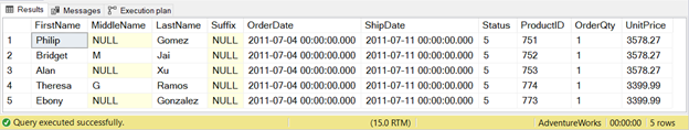
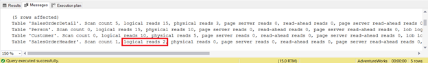
Then, you check the STATISTICS IO result of this query:
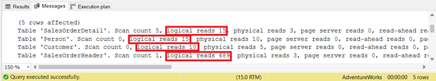
The output shows the logical reads of each of the four tables used in the query. In total, the sum of the logical reads is 729. You can also see physical reads with a total sum of 21. However, but try rerunning the query, and it will be zero.
Take a closer look at the logical reads of SalesOrderHeader. Do you wonder why it has 689 logical reads? Perhaps, you thought of inspecting the below query’s execution plan:
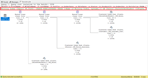
For one thing, there’s an index scan that happened in SalesOrderHeader with a 93% cost. What could be happening? Assume you checked its properties:
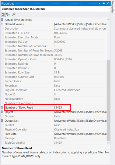
Whoa! 31,465 rows read for only 5 rows returned? It’s absurd!
Reducing the Number of Logical Reads
It’s not so hard to lessen those 31,465 rows read. SQL Server already gave us a clue. Proceed to the following:
STEP 1: Follow SQL Server’s Recommendation and Add the Missing Index
Did you notice the missing index recommendation in the execution plan (Figure 4)? Will that fix the problem?
There’s one way to find out:
CREATE NONCLUSTERED INDEX [IX_SalesOrderHeader_ShipDate]
ON [Sales].[SalesOrderHeader] ([ShipDate])
Rerun the query and see the changes in STATISTICS IO logical reads.
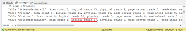
As you can see in STATISTICS IO (Figure 6), there’s a tremendous decrease in logical reads from 689 to 17. The new overall logical reads are 57, which is a significant improvement from 729 logical reads. But to be sure, let’s inspect the execution plan again.
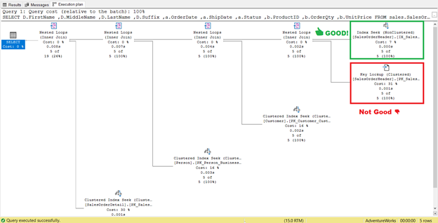
It looks like there’s an improvement in the plan resulting in reduced logical reads. The index scan is now an index seek. SQL Server will no longer need to inspect row-by-row to get the records with the Shipdate=’07/11/2011′. But something is still lurking in that plan, and it’s not right.
You need step 2.
STEP 2: Alter the Index and Add to Included Columns: OrderDate, Status, and CustomerID
Do you see that Key Lookup operator in the execution plan (Figure 7)? It means that the created non-clustered index is not enough – the query processor needs to use the clustered index again.
Let’s check its properties.
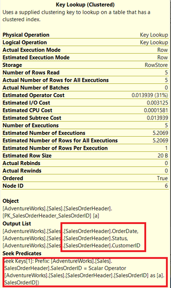
Note the enclosed box under the Output List. It happens that we need OrderDate, Status, and CustomerID in the result set. To obtain those values, the query processor used the clustered index (See the Seek Predicates) to get to the table.
We need to remove that Key Lookup. The solution is to include the OrderDate, Status, and CustomerID columns into the index created earlier.
- Right-click the IX_SalesOrderHeader_ShipDate in SSMS.
- Select Properties.
- Click the Included columns tab.
- Add OrderDate, Status, and CustomerID.
- Click OK.
After recreating the index, rerun the query. Will this remove Key Lookup and reduce logical reads?
It worked! From 17 logical reads down to 2 (Figure 9).
And the Key Lookup?
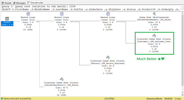
It’s gone! Clustered Index Seek has replaced Key Lookup.
The Takeaway
So, what have we learned?
One of the primary ways to reduce logical reads and improve SQL query performance is to create an appropriate index. But there’s a catch. In our example, it reduced the logical reads. Sometimes, the opposite will be right. It may affect the performance of other related queries too.
Therefore, always check the STATISTICS IO and the execution plan after creating the index.
2. High Lob Logical Reads
It is much the same as point #1, but it will deal with data types text, ntext, image, varchar(max), nvarchar(max), varbinary(max), or columnstore index pages.
Let’s refer to an example: generating lob logical reads.
Example of Lob Logical Reads
Assume you want to display a product with its price, color, thumbnail image, and a larger image on a web page. Thus, you come up with an initial query like as shown below:
SELECT
 a.ProductID
,a.Name AS ProductName
,a.ListPrice
,a.Color
,b.Name AS ProductSubcategory
,d.ThumbNailPhoto
,d.LargePhoto
FROM Production.Product a
INNER JOIN Production.ProductSubcategory b ON a.ProductSubcategoryID = b.ProductSubcategoryID
INNER JOIN Production.ProductProductPhoto c ON a.ProductID = c.ProductID
INNER JOIN Production.ProductPhoto d ON c.ProductPhotoID = d.ProductPhotoID
WHERE b.ProductCategoryID = 1 -- Bikes
ORDER BY ProductSubcategory, ProductName, a.Color
Then, you run it and see the output like the one below:
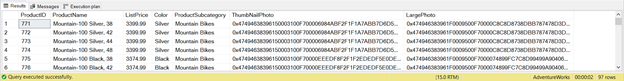
As you are such a high-performance-minded guy (or gal), you immediately check the STATISTICS IO. Here it is:
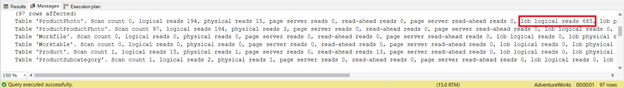
It feels like some dirt in your eyes. 665 lob logical reads? You cannot accept this. Not to mention 194 logical reads each from ProductPhoto and ProductProductPhoto tables. You indeed think this query needs some changes.
Reducing Lob Logical Reads
The previous query had 97 rows returned. All 97 bikes. Do you think that this is good to display on a web page?
An index may help, but why not simplify the query first? This way, you can be selective on what SQL Server will return. You can reduce the lob logical reads.
- Add a filter for the Product Subcategory and let the customer choose. Then include this in the WHERE clause.
- Remove the ProductSubcategory column since you will add a filter for the Product Subcategory.
- Remove the LargePhoto column. Query this when the user selects a specific product.
- Use paging. The customer won’t be able to view all 97 bikes at once.
Based on these operations described above, we change the query as follows:
- Remove ProductSubcategory and LargePhoto columns from the result set.
- Use OFFSET and FETCH to accommodate paging in the query. Query only 10 products at a time.
- Add ProductSubcategoryID in the WHERE clause based on the customer’s selection.
- Remove the ProductSubcategory column in the ORDER BY clause.
The query will now be similar to this:
DECLARE @pageNumber TINYINT
DECLARE @noOfRows TINYINT =  10 -- each page will display 10 products at a time

SELECT
 a.ProductID
,a.Name AS ProductName
,a.ListPrice
,a.Color
,d.ThumbNailPhoto
FROM Production.Product a
INNER JOIN Production.ProductSubcategory b ON a.ProductSubcategoryID = b.ProductSubcategoryID
INNER JOIN Production.ProductProductPhoto c ON a.ProductID = c.ProductID
INNER JOIN Production.ProductPhoto d ON c.ProductPhotoID = d.ProductPhotoID
WHERE b.ProductCategoryID = 1 -- Bikes
AND a.ProductSubcategoryID = 2 -- Road Bikes
ORDER BY ProductName, a.Color
OFFSET (@pageNumber-1)*@noOfRows ROWS FETCH NEXT @noOfRows ROWS ONLY
-- change the OFFSET and FETCH values based on what page the user is.
With the changes done, will lob logical reads improve? STATISTICS IO now reports:
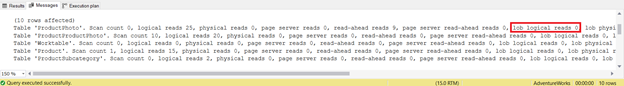
ProductPhoto table now has 0 lob logical reads – from 665 lob logical reads down to none. That is some improvement.
Takeaway
One of the ways to reduce lob logical reads is to rewrite the query to simplify it.
Remove unneeded columns and reduce the returned rows to the least required. When necessary, use OFFSET and FETCH for paging.
To ensure that the query changes have improved lob logical reads and the SQL query performance, always check STATISTICS IO.
3. High Worktable/Workfile Logical Reads
Finally, it’s logical reads of Worktable and Workfile. But what are these tables? Why do they appear when you don’t use them in your query?
Having Worktable and Workfile appearing in the STATISTICS IO means that SQL Server needs a lot more work to get the desired results. It resorts to using temporary tables in tempdb, namely Worktables and Workfiles. It is not necessarily harmful to have them in the STATISTICS IO output, as long as logical reads are zero, and it’s not causing trouble to the server.
These tables may appear when there’s an ORDER BY, GROUP BY, CROSS JOIN, or DISTINCT, among others.
Example of Worktable/Workfile Logical Reads
Assume that you need to query all stores without sales of certain products.
You initially come up with the following:
SELECT DISTINCT
a.SalesPersonID
,b.ProductID
,ISNULL(c.OrderTotal,0) AS OrderTotal
FROM Sales.Store a
CROSS JOIN Production.Product b
LEFT JOIN (SELECT
b.SalesPersonID
,a.ProductID
,SUM(a.LineTotal) AS OrderTotal
FROM Sales.SalesOrderDetail a
INNER JOIN Sales.SalesOrderHeader b ON a.SalesOrderID = b.SalesOrderID
WHERE b.SalesPersonID IS NOT NULL
GROUP BY b.SalesPersonID, a.ProductID, b.OrderDate) c ON a.SalesPersonID
= c.SalesPersonID
AND b.ProductID = c.ProductID
WHERE c.OrderTotal IS NULL
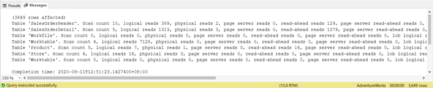
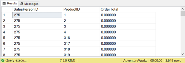
ORDER BY a.SalesPersonID, b.ProductIDThis query returned 3649 rows:
Let’s check what the STATISTICS IO tells:
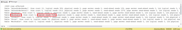
It’s worth notice that the Worktable logical reads are 7128. The overall logical reads are 8853. If you check the execution plan, you’ll see lots of parallelisms, hash matches, spools, and index scans.
Reducing Worktable/Workfile Logical Reads
I could not construct a single SELECT statement with a satisfying result. Thus the only choice is to break down the SELECT statement into multiple queries. See below:
SELECT DISTINCT
 a.SalesPersonID
,b.ProductID
INTO #tmpStoreProducts
FROM Sales.Store a
CROSS JOIN Production.Product b

SELECT
 b.SalesPersonID
,a.ProductID
,SUM(a.LineTotal) AS OrderTotal
INTO #tmpProductOrdersPerSalesPerson
FROM Sales.SalesOrderDetail a
INNER JOIN Sales.SalesOrderHeader b ON a.SalesOrderID = b.SalesOrderID
WHERE b.SalesPersonID IS NOT NULL
GROUP BY b.SalesPersonID, a.ProductID

SELECT
 a.SalesPersonID
,a.ProductID
FROM #tmpStoreProducts a
LEFT JOIN #tmpProductOrdersPerSalesPerson b ON a.SalesPersonID = b.SalesPersonID AND
                                               a.ProductID = b.ProductID
WHERE b.OrderTotal IS NULL
ORDER BY a.SalesPersonID, a.ProductID

DROP TABLE #tmpProductOrdersPerSalesPerson
DROP TABLE #tmpStoreProducts
It’s several lines longer, and it uses temporary tables. Now, let’s see what the STATISTICS IO reveals:
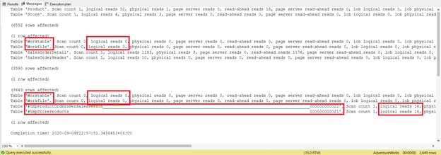
Try not to focus on this statistical report length – it is only frustrating. Instead, add logical reads from each table.
For a total of 1279, it’s a significant decrease, as it was 8853 logical reads from the single SELECT statement.
We haven’t added any index to the temporary tables. You might need one if a lot more records are added to SalesOrderHeader and SalesOrderDetail. But you get the point.
Takeaway
Sometimes 1 SELECT statement appears good. However, behind the scenes, the opposite is true. Worktables and Workfiles with high logical reads lag your SQL query performance.
If you can’t think of another way to reconstruct the query, and the indexes are useless, try the “divide and conquer” approach. The Worktables and Workfiles may still appear in the Message tab of SSMS, but the logical reads will be zero. Therefore, the overall result will be less logical reads.
The Bottomline in SQL Query Performance and STATISTICS IO
What’s the big deal with these 3 nasty I/O statistics?
The difference in SQL query performance will be like night and day if you pay attention to these numbers and lower them. We have only presented some ways to reduce logical reads like:
- creating appropriate indexes;
- simplifying queries – removing unnecessary columns and minimizing the result set;
- breaking down a query into multiple queries.
There are more like updating statistics, defragmenting indexes, and setting the right FILLFACTOR. Can you add more to this in the comment section?
If you like this post, please share it with your favorite social media.
Tags: query performance, sql server, ssms Last modified: September 20, 2021