Analysis of MS SQL Server for Those Who See It for the First Time

What Problems Will We Consider?

If the server notifies “there is no more space on the E drive” – no deep analysis is needed. We will not consider errors, the solution of which is obvious from the text of the message and for which Google immediately throws a link to MSDN with the solution.

Let’s examine the problems which are not obvious for Google, such as, for example, a sudden drop in performance or the absence of connection. Consider the main tools for customization and analysis. Let’s see where the logs and other useful information are located. In fact, I’ll try to collect in one article all the necessary information for a quick start.

First of All

We are going to start with the most frequent questions and consider them separately.

If your database suddenly, for no apparent reason, began to work slowly, but you had not changed anything – first of all, update the statistics and rebuild the indexes.

On the Internet, there are lots of methods like this, examples of scripts are provided. I will assume that all those methods are for professionals. Well, I’ll describe the simplest way: you only need a mouse for implementing it.

Abbreviations

• SSMS is an application of Microsoft SQL Server Management Studio. Starting from the 2016 version, it is available free of charge on the MS website as a standalone application. docs.microsoft.com/en-us/sql/ssms/download-sql-server-management-studio-ssms

• Profiler is an application of “SQL Server Profiler” installed with SSMS.
• Performance Monitor is a snap-in of the control panel that allows you to monitor the performance counters, log and view the history of measurements.

Statistics update using a “service plan”:

• run SSMS;
• connect to a required server;
• expand the tree in Object Inspector: Management\Maintenance Plans (Service Plans);
• right-click the node and select “Maintenance Plan Wizard”;
• in the wizard, mark the required tasks: rebuild index and update statistics

• you can mark both tasks at once or make two maintenance plans with one task in each (see the “important notes” below);
• further, we check a required DB (or several databases). We do this for each task (if two tasks are chosen, there will be two dialogs with the choice of a database);
• Next, Next, Finish.

After these actions, a “maintenance plan” will be created (not executed). You can run it manually by right-clicking it and selecting “Execute”. Alternatively, you configure the launch via SQL Agent.

Important notes:

• Updating statistics is a non-blocking operation. You can perform it in a working mode.
• Index rebuilding is a blocking operation. You can run it only outside the working hours. There is an exception — the Enterprise edition of the server allows the execution of an “online rebuild”. This option can be enabled in the task settings. Please note that there is a checkmark in all the editions, but it works only in Enterprise.
• Of course, these tasks must be performed regularly. I suggest an easy way to determine how often you do this:

– With the first problems, execute the maintenance plan;

– If it helped, wait until the problems occur again (usually until the next monthly closing/salary calculation/ etc. of bulk transactions);

– The resulting period of a normal operation will be your reference point;

– For example, configure the execution of the maintenance plan twice as often.

The Server Is Slow – What Should You Do?

The resources used by the server

Like any other program, the server needs processor time, data on the disk, the amount of RAM, and network bandwidth.

Task Manager will help you assess the lack of a given resource in the first approximation, no matter how terrible it may sound.

CPU Load

Even a schoolboy can check the utilization in the Manager. We just need to make sure that if the processor is loaded, then it’s the sqlserver.exe process.

If this is your case, you need to go to the analysis of user activity to understand what exactly caused the load (see below).

Disc Load

Many people only look at the CPU load but forget that the DBMS is a data store. The data volumes are growing, the processor performance is increasing while the HDD speed is pretty much the same. With SSDs the situation is better, but storing terabytes on them is expensive.

It turns out that I often encounter situations where the disk system becomes the bottleneck, rather than the CPU.

For disks, the following metrics are important:

• average queue length (outstanding I/O operations, number);
• read-write speed (in Mb/s).

The server version of the Task Manager, as a rule (depending on the system version), shows both. If not, run the Performance Monitor snap-in (system monitor). We are interested in the following counters:

• Physical (logical) disk/Average read (write) time
• Physical (logical) disk/Average disk queue length
• Physical (logical) disk/Disk speed

For more details, you can read the manufacturer’s manuals, for example, here: social.technet.microsoft.com/wiki/contents/articles/3214.monitoring-disk-usage.aspx.

In short:

• The queue should not exceed 1. Short bursts are allowed if they quickly subside. The bursts can be different depending on your system. For a simple RAID mirror of two HDDs – the queue of more than 10-20 is a problem. For a cool library with super caching, I saw bursts of up to 600-800 which were instantly resolved without causing delays.
• The normal exchange rate also depends on the type of a disk system. The usual (desktop) HDD transmits at 50-100 MB/s. A good disk library – at 500 MB/s and more. For small random operations, the speed is less. This may be your reference point.
• These parameters must be considered as a whole. If your library transmits 50MB/s and a queue of 50 operations lines up — obviously, something is wrong with the hardware. If the queue lines up when the transmission is close to a maximum – most likely, the disks are not to be blamed for – they just cannot do more – we need to look for a way to reduce the load.
• The load should be checked separately on disks (if there are several of them) and compared with the location of server files. The Task Manager can show the most actively used files. This can be used to ensure that the load is caused by DBMS.

What can cause the disk system problems:

• problems with hardware

• cache burned out, performance dropped dramatically;
• the disk system is used by something else;

• RAM shortage. Swapping. Сaching decayed, performance dropped (see the section about RAM below).
• User load increased. It is necessary to evaluate the work of users (problematic query/new functionality/increase in the number of users/increase in the amount of data/etc).
• Database data fragmentation (see the index rebuild above), system files fragmentation.
• The disk system has reached its maximum capabilities.

In the case of the last option – do not throw out the hardware at once. Sometimes, you can get a little more out of the system if you approach the problem wisely. Check the location of the system files for compliance with the recommended requirements:

• Do not mix OS files with database data files. Store them on different physical media so that the system does not compete with DBMS for I/O.
• The database consists of two file types: data (*.mdf, *.ndf) and logs (*.ldf).
  Data files, as a rule, are mostly used for reading. Logs serve for writing (wherein the writing is consecutive). It is, therefore, recommended to store logs and data on different physical media so that the logging does not interrupt the data reading (as a rule, the write operation takes precedence over reading).
• MS SQL can use “temporary tables” for query processing. They are stored in the tempdb system database. If you have a high load on files of this database, you can try to render it on physically separate media.

Summarizing the issue with file location, use the principle of “divide and conquer”. Evaluate which files are accessed and try to distribute them to different media. Also, use the features of RAID systems. For example, RAID-5 reads are faster than writes – which is good for data files.

Let’s explore how to retrieve information about user performance: who makes what, and how much resources are consumed

I divided tasks of auditing user activity into the following groups:

1. Tasks of analyzing particular request.
2. Tasks of analyzing load from the application in specific conditions (for example, when a user clicks a button in a third-party application compatible with the database).
3. Tasks of analyzing the current situation.

Let’s consider each of them in detail.

Warning

The performance analysis requires a deep understanding of the structure and principles of operation of the database server and operating system. That’s why the reading of only these articles will not make you a professional.

The considered criteria and counters in real systems depend on each other greatly. For example, a high HDD load is often caused by a lack of RAM. Even if you conduct some measurements, this is not enough to assess the problems reasonably.

The purpose of the articles is to introduce the essentials on simple examples. You should not consider my recommendations as a guide. I recommend you use them as training tasks that can explain the flow of thoughts.

I hope that you will learn how to rationalize your conclusions about the server performance in figures.

Instead of saying “server slows down”, you will provide specific values of specific indicators.

Analyze a Particular Request

The first point is quite simple, let’s dwell on it briefly. We will consider some less obvious issues.

In addition to query results, SSMS allows retrieving additional information about the query execution:

• You can obtain the query plan by clicking the “Display Estimated Execution Plan” and “Include Actual Execution Plan” buttons. The difference between them is that the estimation plan is built without a query execution. Thus, the information about the number of processed rows will be estimated. In the actual plan, there will be both, estimated and actual data. Strong discrepancies of these values indicate that the statistics are not relevant. However, the analysis of the plan is a subject for another article – so far, we will not go deeper.
• We can get measurements of processor costs and disk operations of the server. To do this, it is necessary to enable the SET option. You can do it either in the ‘Query options’ dialog box like this:

Or with the direct SET commands in the query: 

      SET STATISTICS IO ON
      SET STATISTICS TIME ON
      SELECT * FROM Production.Product p
      JOIN Production.ProductDocument pd ON p.ProductID = pd.ProductID
      JOIN Production.ProductProductPhoto ppp ON p.ProductID = ppp.ProductID

As a result, we will get data on the time spent on compilation and execution, as well as the number of disk operations.

Time of SQL Server parsing and compilation:
CPU time = 16 ms, elapsed time = 89 ms.
 
SQL Server performance time:
CPU time = 0 ms, time spent = 0 ms.
 
SQL Server performance time:
CPU time = 0 ms, time spent = 0 ms.
(32 row(s) affected)
The «ProductProductPhoto» table. The number of views is 32, logic reads – 96, physical reads 5, read-ahead reads 0, lob of logical reads 0, lob of physical reads 0, lob of read-ahead reads 0.
The ‘Product’ table. The number of views is 0, logic reads – 64, physical reads – 0, read-ahead reads – 0, lob of logical reads – 0, lob of physical reads – 0, lob of readahead reads – 0.
The «ProductDocument» table. The number of views is 1, logical reads – 3, physical reads – 1, read-ahead reads -, lob of logical reads – 0, lob of physical reads – 0, lob of readahead reads – 0.
Time of SQL activity:
CPU time = 15 ms, spent time = 35 ms.

I would like to draw your attention to the compilation time, logical reads 96, and physical reads 5. When executing the same query for the second time and later, physical reads may decrease, and recompilation may not be required. Due to this fact, it often happens that the query is executed faster during the second and subsequent times than for the first time. The reason, as you understand, is in caching the data and compiled query plans.

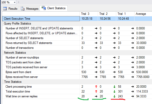
• The «Include Client Statistics» button displays the information on network exchange, the amount of executed operations and total execution time, including the costs on network exchange and processing by a client. The example shows that it takes more time to execute the query for the first time:

• In SSMS 2016, there is the «Include Live Query Statistics» button. It displays the image as in the case of the query plan but contains the nonrandom digits of the processed rows, which change on the screen while executing the query. The picture is very clear – flashing arrows and running numbers, you can immediately see where the time is wasted. The button also works for SQL Server 2014 and later.

To sum up:

• Check the CPU costs using SET STATISTICS TIME ON.
• Disk operations: SET STATISTICS IO ON. Do not forget that logic read is a read operation completed in the disk cache without physically accessing the disk system. “Physical read” takes much more time.
• Evaluate the volume of network traffic using «Include Client Statistics».
• Analyze the algorithm of executing the query by the execution plan using «Include Actual Execution Plan» and «Include Live Query Statistics».

Analyze the Application Load

Here we will use SQL Server Profiler. After launching and connecting to the server, it is necessary to select log events. To do this, run profiling with a standard tracing template. On the General tab in the Use the template field, select Standard (default) and click Run.

The more complicated way is to add/drop filters or events to/from the selected template. These options may be found on the second tab of the dialog menu. To see the full range of possible events and columns to select, select the Show All Events and Show All Columns checkboxes.

We will need the following events:

• Stored Procedures \ RPC:Completed
• TSQL \ SQL:BatchCompleted

These events monitor all external SQL calls to the server. They appear after the completion of the query processing. There are similar events that keep track of the SQL Server start:

• Stored Procedures \ RPC:Starting
• TSQL \ SQL:BatchStarting

However, we do not need these procedures as they do not contain information about the server resources spent on the query execution. It is obvious that such information is available only after the completion of the execution process. Thus, columns with data on CPU, Reads, Writes in the *Starting events will be empty.

The following events may interest us as well, however, we will not enable them so far:

• Stored Procedures \ SP:Starting (*Completed) monitors the internal call to the stored procedure not from the client, but within the current request or other procedure.
• Stored Procedures \ SP:StmtStarting (*Completed) tracks the start of each statement within the stored procedure. If there is a cycle in the procedure, the number of events for the commands in the cycle will equal the number of iterations in the cycle.
• TSQL \ SQL:StmtStarting (*Completed) monitors the start of each statement within the SQL-batch. If there are several commands in your query, each of them will contain one event. Thus, it works for the commands located in the query.

These events are convenient for monitoring the execution process.

By Columns

Which columns to select is clear from the button name. We will need the following ones:

• TextData, BinaryData contain the query text.
• CPU, Reads, Writes, Duration display resource consumption data.
• StartTime, EndTime is the time to start and finish the execution process. They are convenient for sorting.

Add other columns based on your preferences.

The Column Filters… button opens the dialog box for configuring event filters. If you are interested in the activity of the particular user, you can set the filter by the SID number or username. Unfortunately, in the case of connecting the app through the app-server with the pull of connections, monitoring of the particular user becomes more complicated.

You can use filters for the selection of only complicated queries (Duration>X), queries that cause intensive write (Writes>Y), as well as query content selections, etc.

What else do we need from the profiler? Of course, the execution plan!

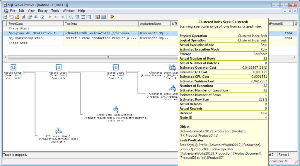
It is necessary to add the «Performance \ Showplan XML Statistics Profile» event to the tracing. While executing our query, we will get the following image:

The query text:

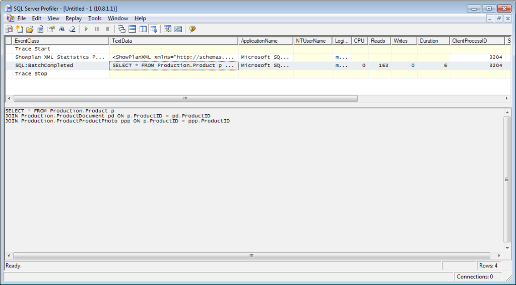
The execution plan:

And that Is Not All

It is possible to save a trace to a file or a database table. Tracing settings can be stored as a personal template for a quick run. You can run the trace without a profiler, by simply using a T-SQL code, and the sp_trace_create, sp_trace_setevent, sp_trace_setstatus, sp_trace_getdata procedures. You can find an example here. This approach can be useful, for example, to automatically start storing a trace to a file on a schedule.  You can have a sneaky peak at the profiler to see how to use these commands. You can run two traces and in one of them track what happens when the second one starts. Check that there is no filter by the “ApplicationName” column on the profiler itself.

The list of the events monitored by the profiler is very large and is not limited to receiving query texts. There are events that track fullscan, recompiling, autogrow, deadlock, and much more.

Analyzing User Activity on the Server

There are different situations. A query can hang on ‘execution’ for a long time and it is unclear whether it will be completed or not. I would like to analyze the problematic query separately; however, we must first determine what the query is. It’s useless to catch it with a profiler – we have already missed the starting event, and it’s not clear how long to wait for the process to be completed.

Let’s figure it out

You might have heard about ‘Activity Monitor’. Its higher editions have really rich functionality. How can it help us? Activity Monitor includes many useful and interesting features. We will get everything we need from system views and functions. Monitor itself is useful because you can set the profiler on it and see what queries it performs.

We will need:

• dm_exec_sessions provides information about sessions of connected users. Within our article, the useful fields are those that identify a user (login_name, login_time, host_name, program_name, …) and fields with the information on spent resources (cpu_time, reads, writes, memory_usage, …)
• dm_exec_requests provides information about queries executed at the moment.
• session_id is an identifier of the session to link to the previous view.
• start_time is the time for the view run.
• command is a field that contains a type of the executed command. For user queries, it is select/update/delete/
• sql_handle, statement_start_offset, statement_end_offset provide information for retrieving query text: handle, as well as the start and finish position in the text of the query, which means the part that is currently being executed (for the case when your query contains several commands).
• plan_handle is a handle of the generated plan.
• blocking_session_id indicates the number of the session that caused blocking if there are blocks that prevent the execution of the query
• wait_type, wait_time, wait_resource are fields with the information about the reason and duration of the wait. For some types of waits, for example, data lock, it is necessary to indicate additionally a code for the blocked resource.
• percent_complete is the percentage of completion. Unfortunately, it is only available for commands with a clearly predictable progress (for example, backup or restore).
• cpu_time, reads, writes, logical_reads, granted_query_memory are resource costs.
• dm_exec_sql_text(sql_handle | plan_handle), sys.dm_exec_query_plan(plan_handle) are functions of getting the text and execution plan. Below, we will consider an example of its use.
• dm_exec_query_stats is a summary statistics of executing queries. It displays the query, the number of its executions, and the volume of spent resources.

Important Notes

The above list is just a small part. A complete list of all system views and functions is described in the documentation. Also, there is a beautiful image showing a diagram of links between the main objects.

The query text, its plan, and execution statistics are data stored in the procedure cache. They are available during execution. Then, availability is not guaranteed and depends on the cache load. Yes, the cache can be manually cleaned. Sometimes, it is recommended when the execution plans ‘flipped out’. Still, there are a lot of nuances.

The “command” field is meaningless for user requests, as we can get the full text. However, it is very important for obtaining information about system processes. As a rule, they perform some internal tasks and do not have the SQL text. For such processes, the information about the command is the only hint of the activity type.

In the comments to the previous article, there was a question about what the server is involved in when it should not work. The answer will probably be in the meaning of this field. In my practice, the “command” field always provided something quite understandable for active system processes: autoshrink / autogrow / checkpoint / logwriter / etc.

How to Use It

We will go to the practical part. I will provide several examples of its use. Server possibilities are not limited – you can think of your own examples.

Example 1. What process consumes CPU/reads/writes/memory

First, have a look at the sessions that consume more resources, for example, CPU. You may find this information in sys.dm_exec_sessions. However, data on CPU, including reads and writes, is cumulative. It means that the number contains the total for all the time of connection. It is clear that the user who connected a month ago and was not disconnected will have a higher value. It does not mean that they overload the system.

A code with the following algorithm may solve this problem:

1. Make a selection and store it in a temporary table
2. Wait for some time
3. Make a selection for the second time
4. Compare these results. Their difference will indicate costs spent at step 2.
5. For convenience, the difference can be divided by the duration of step 2 in order to obtain the average “costs per second”.

if object_id('tempdb..#tmp') is NULL
BEGIN
        SELECT * into #tmp from sys.dm_exec_sessions s
        PRINT 'wait for a second to collect statistics at the first run '
        -- we do not wait for the next launches, because we compare with the result of the previous launch
        WAITFOR DELAY '00:00:01';
END
if object_id('tempdb..#tmp1') is not null drop table #tmp1

declare @d datetime
declare @dd float
select @d = crdate from tempdb.dbo.sysobjects where id=object_id('tempdb..#tmp')

select * into #tmp1 from sys.dm_exec_sessions s
select @dd=datediff(ms,@d,getdate())
select @dd AS [time interval, ms]

SELECT TOP 30 s.session_id, s.host_name, db_name(s.database_id) as db, s.login_name,s.login_time,s.program_name,
       s.cpu_time-isnull(t.cpu_time,0) as cpu_Diff, convert(numeric(16,2),(s.cpu_time-isnull(t.cpu_time,0))/@dd*1000) as cpu_sec,
       s.reads+s.writes-isnull(t.reads,0)-isnull(t.writes,0) as totIO_Diff, convert(numeric(16,2),(s.reads+s.writes-isnull(t.reads,0)-isnull(t.writes,0))/@dd*1000) as totIO_sec,
       s.reads-isnull(t.reads,0) as reads_Diff, convert(numeric(16,2),(s.reads-isnull(t.reads,0))/@dd*1000) as reads_sec,
       s.writes-isnull(t.writes,0) as writes_Diff, convert(numeric(16,2),(s.writes-isnull(t.writes,0))/@dd*1000) as writes_sec,
       s.logical_reads-isnull(t.logical_reads,0) as logical_reads_Diff, convert(numeric(16,2),(s.logical_reads-isnull(t.logical_reads,0))/@dd*1000) as logical_reads_sec,
       s.memory_usage, s.memory_usage-isnull(t.memory_usage,0) as [mem_D],
      s.nt_user_name,s.nt_domain
from #tmp1 s
LEFT join #tmp t on s.session_id=t.session_id
order BY
cpu_Diff desc
--totIO_Diff desc
--logical_reads_Diff desc

drop table #tmp
GO
select * into #tmp from #tmp1
drop table #tmp1

I use two tables in the code:  #tmp – for the first selection, and #tmp1 – for the second one. During the first run, the script creates and fills #tmp and #tmp1 at an interval of one second, and then performs other tasks. With the next runs, the script uses the results of the previous execution as a base for comparison. Thus, the duration of step 2 will be equal to the duration of your wait between the script runs.

Try executing it, even on the production server.  The script will create only ‘temporary tables’ (available within the current session and deleted when disabled) and has no thread.

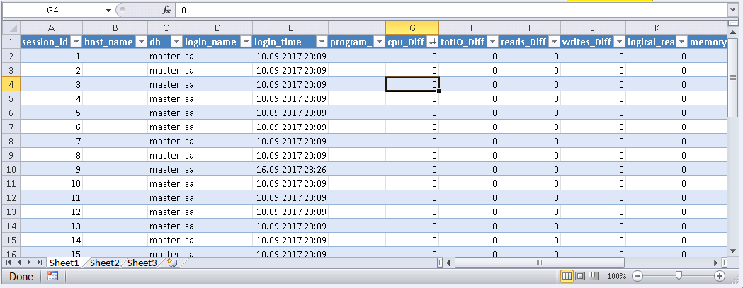
Those who do not like to execute a query in MS SSMS can wrap it in an application written in their favorite programming language. I’ll show you how to do this in MS Excel without a single line of code.

In the Data menu, connect to the server. If you are prompted to select a table, select a random one. Click Next and Finish until you see the Data Import dialog. In that window, you need to click Properties. In Properties, it is necessary to replace a command type with the SQL value and insert our modified query in the Command text field.

You will have to modify the query a little bit:

• Add «SET NOCOUNT ON»
• Replace temporary tables with variable tables
• Delay will last within 1 sec. Fields with averaged values are not required

The modified Query for Excel

SET NOCOUNT ON;
declare @tmp table(session_id   smallint primary key,login_time datetime,host_name nvarchar(256),program_name nvarchar(256),login_name nvarchar(256),nt_user_name       nvarchar(256),cpu_time  int,memory_usage        int,reads       bigint,writes   bigint,logical_reads    bigint,database_id      smallint)

declare @d datetime;
select @d=GETDATE()

INSERT INTO @tmp(session_id,login_time,host_name,program_name,login_name,nt_user_name,cpu_time,memory_usage,reads,writes,logical_reads,database_id)
SELECT session_id,login_time,host_name,program_name,login_name,nt_user_name,cpu_time,memory_usage,reads,writes,logical_reads,database_id
from sys.dm_exec_sessions s;

WAITFOR DELAY '00:00:01';

declare @dd float;
select @dd=datediff(ms,@d,getdate());

SELECT 
        s.session_id, s.host_name, db_name(s.database_id) as db, s.login_name,s.login_time,s.program_name,
        s.cpu_time-isnull(t.cpu_time,0) as cpu_Diff,
        s.reads+s.writes-isnull(t.reads,0)-isnull(t.writes,0) as totIO_Diff,
        s.reads-isnull(t.reads,0) as reads_Diff,
        s.writes-isnull(t.writes,0) as writes_Diff,
        s.logical_reads-isnull(t.logical_reads,0) as logical_reads_Diff,
        s.memory_usage, s.memory_usage-isnull(t.memory_usage,0) as [mem_Diff],
        s.nt_user_name,s.nt_domain
from sys.dm_exec_sessions s
left join @tmp t on s.session_id=t.session_id

Result:

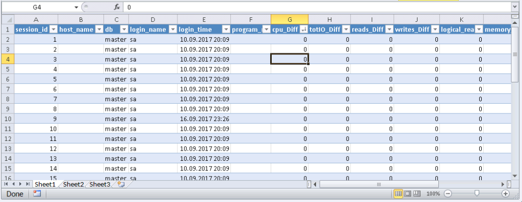
When data appears in Excel, you can sort it, as you need. To update the information, click ‘Refresh’. In the workbook settings, you can put “auto-update” in a specified period of time and “update at the start”. You can save the file and pass it to your colleagues. Thus, we created a convenient and simple tool.

Example 2. What does a session spend resources on?

Now, we are going to determine what the problem sessions actually do. To do this, use sys.dm_exec_requests and functions to receive query text and query plan.

The query and execution plan by the session number

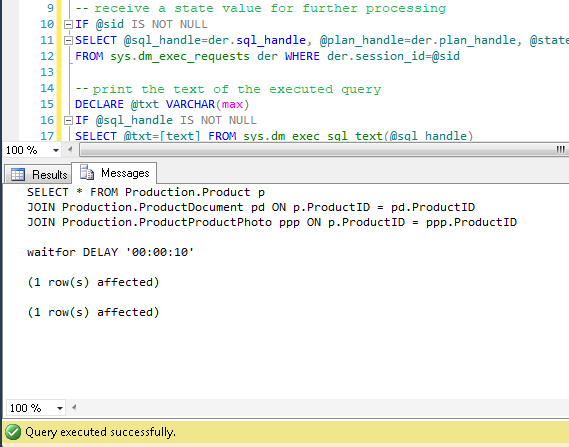
DECLARE @sql_handle varbinary(64)
DECLARE @plan_handle varbinary(64)
DECLARE @sid INT
Declare @statement_start_offset int, @statement_end_offset INT, @session_id SMALLINT

-- for the information by a particular user – indicate a session number
SELECT @sid=182

-- receive state variables for further processing
IF @sid IS NOT NULL
SELECT @sql_handle=der.sql_handle, @plan_handle=der.plan_handle, @statement_start_offset=der.statement_start_offset, @statement_end_offset=der.statement_end_offset, @session_id = der.session_id
FROM sys.dm_exec_requests der WHERE der.session_id=@sid

-- print the text of the query being executed 
DECLARE @txt VARCHAR(max)
IF @sql_handle IS NOT NULL
SELECT @txt=[text] FROM sys.dm_exec_sql_text(@sql_handle)
PRINT @txt
-- output the plan of the batch/procedure being executed
IF @plan_handle IS NOT NULL
select * from sys.dm_exec_query_plan(@plan_handle)
-- and the plan of the query being executed within the batch/procedure
IF @plan_handle IS NOT NULL
SELECT dbid, objectid, number, encrypted, CAST(query_plan AS XML) AS planxml
from sys.dm_exec_text_query_plan(@plan_handle, @statement_start_offset, @statement_end_offset)

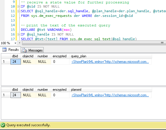
Insert the session number into the query and run it. After execution, there will be plans on the Results tab (the first one is for the whole query, and the second one is for the current step if there are several steps in the query) and the query text on the Messages tab. To view the plan, you need to click the text that looks like the URL in the row. The plan will be opened in a separate tab. Sometimes, it happens that the plan is opened not in a graphical form, but in the form of XML-text. This may happen because the MS SSMS version is lower than the server. Delete the “Version” and “Build” from the first row and then save the result XML to a file with the .sqlplan extension. After that, open it separately. If this does not help, I remind you that the 2016 studio is officially available for free on the MS website.

It is obvious that the result plan will be an estimated one, as the query is being executed. Still, it is possible to receive some execution statistics. To do this, use the sys.dm_exec_query_stats view with the filter by our handles.

Add this information at the end of the previous query

-- plan statistics 
IF @sql_handle IS NOT NULL
SELECT * FROM sys.dm_exec_query_stats QS WHERE QS.sql_handle=@sql_handle

As a result, we will get the information about the steps of the executed query: how many times they were executed and what resources were spent. This information is added to the statistics only after the execution process is completed. The statistics are not tied to the user but are maintained within the whole server. If different users execute the same query, the statistics will be total for all users.

Example 3. Can I see all of them?

Let’s combine the system views we considered with the functions in one query. It can be useful for evaluating the whole situation.

-- receive a list of all current queries
SELECT LEFT((SELECT [text] FROM sys.dm_exec_sql_text(der.sql_handle)),500) AS txt
--,(select top 1 1 from sys.dm_exec_query_profiles where session_id=der.session_id) as HasLiveStat
,der.blocking_session_id as blocker, DB_NAME(der.database_id) AS База, s.login_name, *
from sys.dm_exec_requests der
left join sys.dm_exec_sessions s ON s.session_id = der.session_id
WHERE der.session_id<>@@SPID
-- AND der.session_id>50

The query outputs a list of active sessions and texts of their queries. For system processes, usually, there is no query; however, the command field is filled up. You can see the information about blocks and waits, and mix this query with example 1 in order to sort by the load. Still, be careful, query texts may be large. Their massive selection can be resource-intensive and lead to a huge traffic increase. In the example, I limited the result query to the first 500 characters but did not execute the plan.

Conclusion

It would be great to get Live Query Statistics for an arbitrary session. According to the manufacturer, now, monitoring statistics requires many resources and therefore, it is disabled by default. Its enabling is not a problem, but additional manipulations complicate the process and reduce the practical benefit.

In this article, we analyzed user activity in the following ways: using possibilities MS SSMS, profiler, direct calls to system views. All these methods allow estimating costs on executing a query and getting the execution plan. Each method is suitable for a particular situation. Thus, the best solution is to combine them.

Tags: database administration, performance, sql server, ssms Last modified: September 24, 2021