Problem
In this article, we will focus on the demonstration of table partitioning. The simplest explanation of table partitioning can be called dividing large tables into small ones. This topic provides scalability and manageability.
What is table partitioning in SQL Server?
Assume that we have a table and it grows day by day. In this case, the table can cause some problems which need to be solved by the steps defined below:
- Maintain this table. It will take a long time and consume more resources (CPU, IO etc.).
- Back up.
- Lock problems.
Due to above-mentioned reasons, we need a table partitioning. This approach has the following benefits:
- Management capability: If we break the table apart, we can manage each partition of the table. For example, we can make only one partition of the table.
- Archiving capability: Some partitions of the table are used only for this reason. We don’t need to back up this partition of the table. We can use a filegroup backup and back up it only by changing a partition of the table.
- Query performance: SQL Server query optimizer decides to use partition elimination. It means that SQL Server does not make any search for the unrelated partition of the table.
Vertical and Horizontal Table Partitioning in SQL Server
Table partitioning is a general concept. There are several partitioning types that work for particular cases. The most essential and widely used are the two approaches: vertical partitioning and horizontal partitioning.
The specificity of each type reflects the essence of a table as a structure consisting of columns and rows:
• Vertical Partitioning splits the table into columns.
• Horizontal Partitioning splits the table into rows.
The vertical table partitioning most typical example is a table of employees with their details – names, emails, phone numbers, addresses, birthdays, occupations, salaries, and all other information that might be needed. A part of such data is confidential. Besides, in most cases, operators only need some basic data like names and email addresses.
The vertical partitioning creates several “narrower” tables with the necessary data at hand. Queries target a specific part only. This way, businesses reduce the load, accelerate the tasks, and ensure that confidential data won’t be revealed.
The horizontal table partitioning results in splitting one general table into several smaller ones, where each particle table has the same number of columns, but the number of rows is fewer. It is a standard approach for excessive tables with chronological data.
For instance, a table with the data for the whole year can be divided into smaller sections for each month or week. Then, the query will only concern one specific smaller table. Horizontal partitioning improves the scalability for the data volumes with their growth. The partitioned tables will remain smaller and easy to process.
Any table partitioning in SQL server should be considered with care. Sometimes you have to request the data from several partitioned tables at once, and then you’ll need JOINs in queries. Besides, vertical partitioning may still result in large tables, and you will have to split them more. In your work, you should rely on the decisions for your specific business purposes.
Now that we have clarified the concept of the table partitioning in SQL Server, it’s time to proceed to the demonstration.
We are going to avoid any T-SQL script and handle all the table partition steps with the SQL Server Partitioning wizard.
What do you need to make SQL database partitions?
- WideWorldImporters Sample Database
- SQL Server 2017 Developer Edition
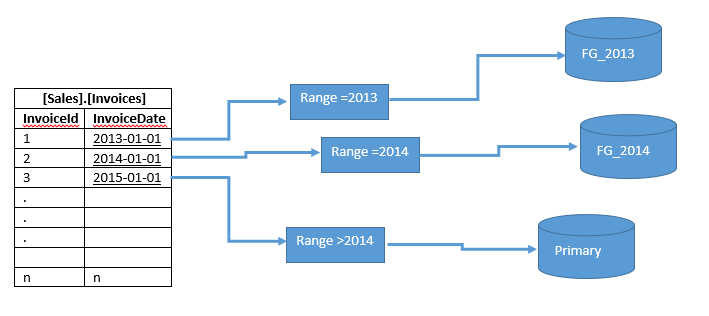
The below image shows us how to design a table partition. We will make a table partition by years and locate different filegroups.
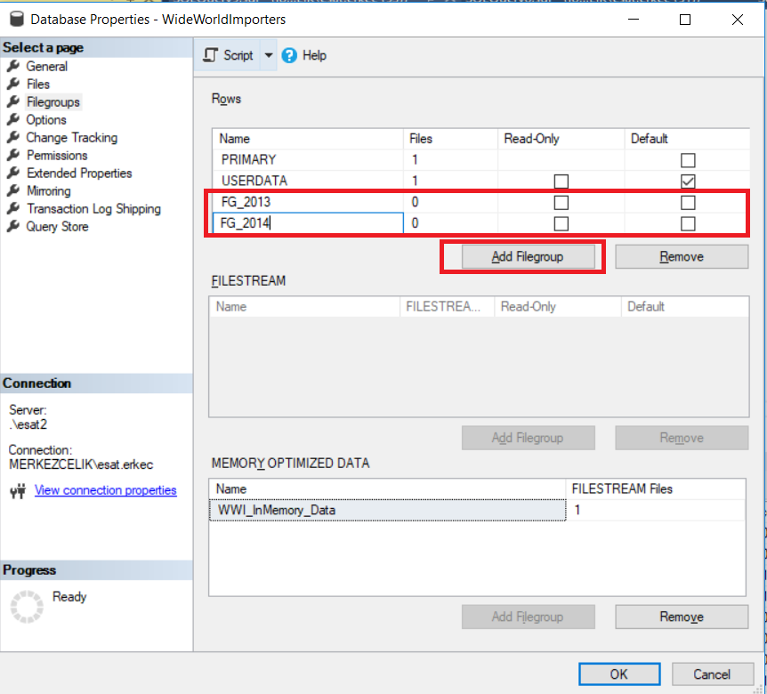
At this step, we will create two filegroups (FG_2013, FG_2014). Right-click a database and then click the Filegroups tab.
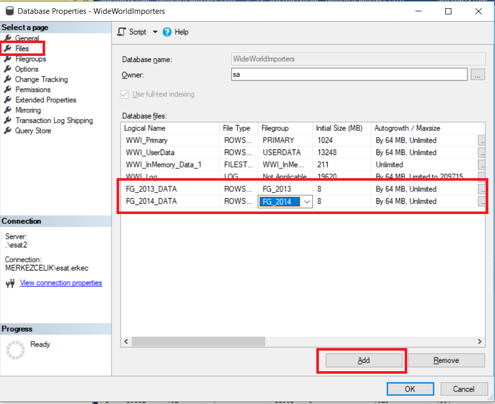
Now, we will connect the file groups to new pdf files.
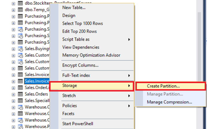
Our database storage structure is ready for table partitioning. We will locate the table which we want to be partitioned and start the Create Partition wizard.
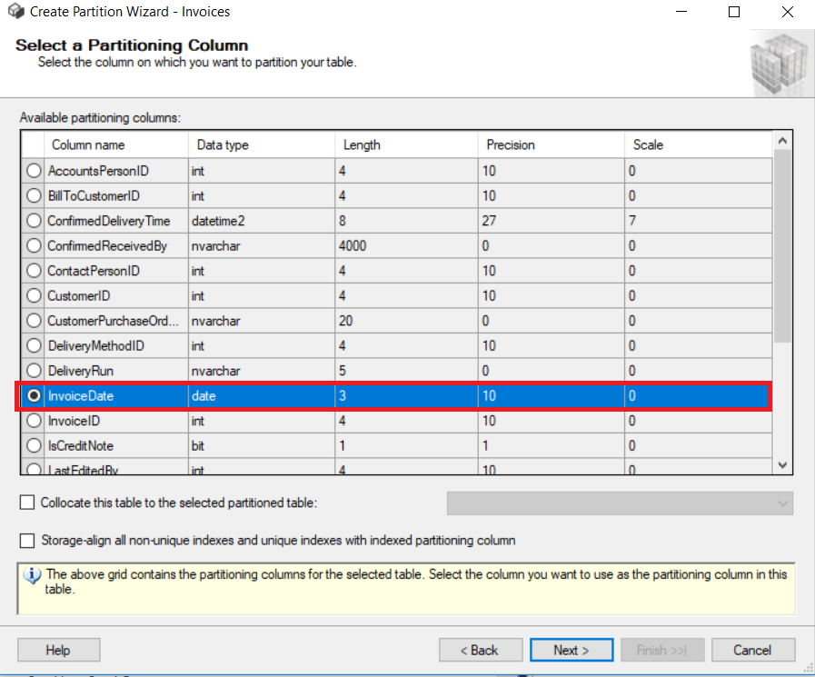
On the screenshot below, we will select a column that we want to apply the partition function on. The selected column is “InvoiceDate”.
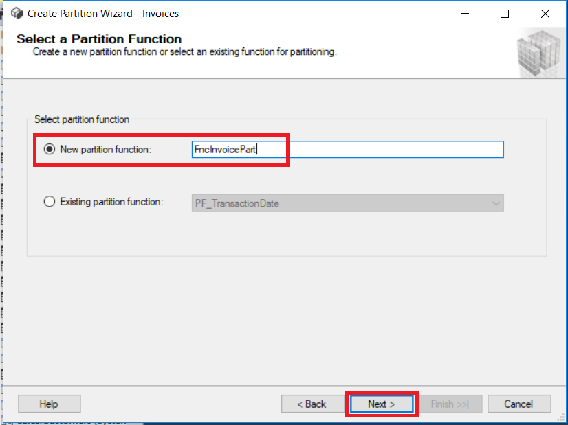
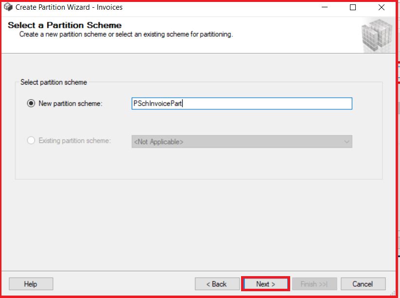
On the next two screens, we will name a partition function and a partition scheme.
A partition function will define how to do partition for the [Sales].[Invoices] rows based on the InvoiceDate column.
A partition scheme will define maps for the Sales.Invoices rows to filegroups.
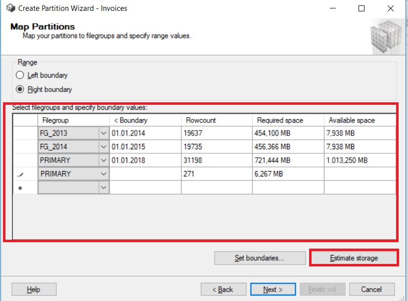
Assign the partitions to filegroups and set the boundaries.
Left /Right Boundary defines the side of each boundary value interval which may be left or right. We will set boundaries like this and click Estimate storage. This option provides us with the information about the number of rows to be located in the boundaries.
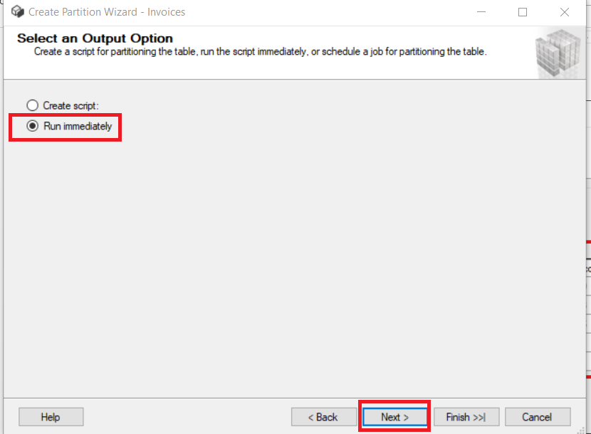
And finally, we will select Run immediately and then click Next.
Once the operation is successful, click Close.
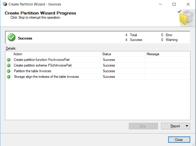
As you can see, our Sales.Invoices table has been partitioned. This query will show the details of the partitioned table.
SELECT
  OBJECT_SCHEMA_NAME(pstats.object_id) AS SchemaName
  ,OBJECT_NAME(pstats.object_id) AS TableName
  ,ps.name AS PartitionSchemeName
  ,ds.name AS PartitionFilegroupName
  ,pf.name AS PartitionFunctionName
  ,CASE pf.boundary_value_on_right WHEN 0 THEN 'Range Left' ELSE 'Range Right' END AS PartitionFunctionRange
  ,CASE pf.boundary_value_on_right WHEN 0 THEN 'Upper Boundary' ELSE 'Lower Boundary' END AS PartitionBoundary
  ,prv.value AS PartitionBoundaryValue
  ,c.name AS PartitionKey
  ,CASE
    WHEN pf.boundary_value_on_right = 0
    THEN c.name + ' > ' + CAST(ISNULL(LAG(prv.value) OVER(PARTITION BY pstats.object_id ORDER BY pstats.object_id, pstats.partition_number), 'Infinity') AS VARCHAR(100)) + ' and ' + c.name + ' <= ' + CAST(ISNULL(prv.value, 'Infinity') AS VARCHAR(100))
    ELSE c.name + ' >= ' + CAST(ISNULL(prv.value, 'Infinity') AS VARCHAR(100))  + ' and ' + c.name + ' < ' + CAST(ISNULL(LEAD(prv.value) OVER(PARTITION BY pstats.object_id ORDER BY pstats.object_id, pstats.partition_number), 'Infinity') AS VARCHAR(100))
  END AS PartitionRange
  ,pstats.partition_number AS PartitionNumber
  ,pstats.row_count AS PartitionRowCount
  ,p.data_compression_desc AS DataCompression
FROM sys.dm_db_partition_stats AS pstats
INNER JOIN sys.partitions AS p ON pstats.partition_id = p.partition_id
INNER JOIN sys.destination_data_spaces AS dds ON pstats.partition_number = dds.destination_id
INNER JOIN sys.data_spaces AS ds ON dds.data_space_id = ds.data_space_id
INNER JOIN sys.partition_schemes AS ps ON dds.partition_scheme_id = ps.data_space_id
INNER JOIN sys.partition_functions AS pf ON ps.function_id = pf.function_id
INNER JOIN sys.indexes AS i ON pstats.object_id = i.object_id AND pstats.index_id = i.index_id AND dds.partition_scheme_id = i.data_space_id AND i.type <= 1 /* Heap or Clustered Index */
INNER JOIN sys.index_columns AS ic ON i.index_id = ic.index_id AND i.object_id = ic.object_id AND ic.partition_ordinal > 0
INNER JOIN sys.columns AS c ON pstats.object_id = c.object_id AND ic.column_id = c.column_id
LEFT JOIN sys.partition_range_values AS prv ON pf.function_id = prv.function_id AND pstats.partition_number = (CASE pf.boundary_value_on_right WHEN 0 THEN prv.boundary_id ELSE (prv.boundary_id+1) END)
WHERE pstats.object_id = OBJECT_ID('Sales.Invoices')
ORDER BY TableName, PartitionNumber;

MS SQL Server partitioning performance
We will compare the partitioned and non-partitioned table performance for the same table. To do this, use the below query and activate Include Actual Execution Plan.
DECLARE @Dt as date  = '20131231'
SELECT COUNT(InvoiceDate)
  FROM [Sales].[Invoices]
  where InvoiceDate < @Dt
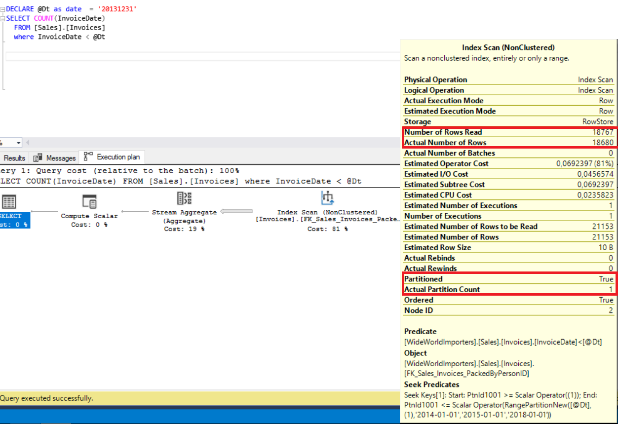
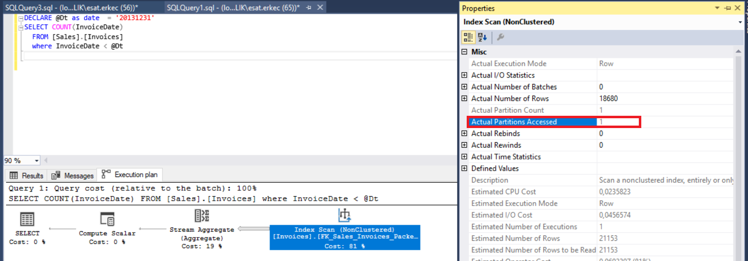
When we examine the execution plan, we come to know that it includes “Partitioned”, “Actual Partition Count”, and “Actual Partitioned Accessed” properties.
The Partitioned property indicates that this table is enabled for partition.
The Actual Partition Count property is the total number of partitions which are read by SQL Server engine.
The Actual Partitioned Accessed property is partition numbers assessed by SQL Server engine. SQL Server eliminates the access for other partitions as it is called a partition elimination and gains an advantage on query performance.
Now, look at the non-partitioned table execution plan.
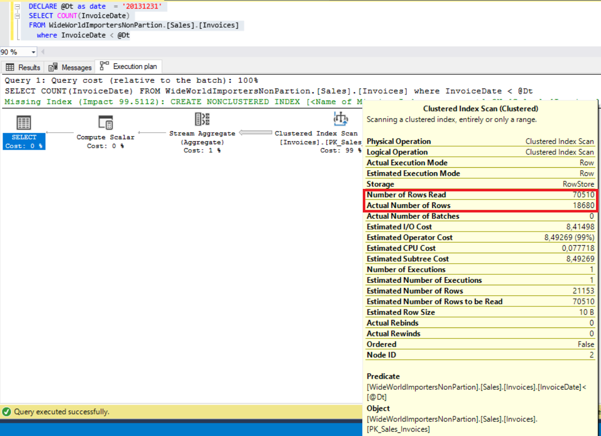
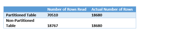
The main difference between these two execution plans is Number of Rows Read because this property indicates how many rows are read for this query. As you can see from the below compression chart, partitioned table values are too low. For this reason, it will consume a low IO.
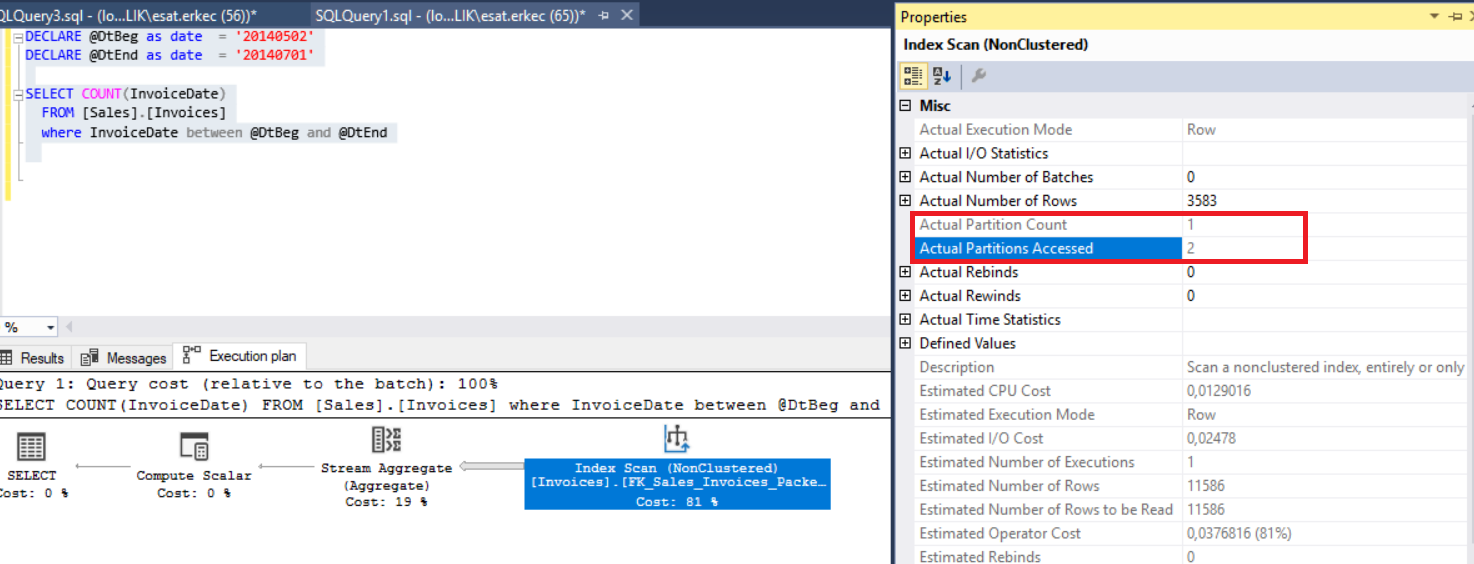
Next, run the query and examine the execution plan.
DECLARE @DtBeg as date  = '20140502'
DECLARE @DtEnd as date  = '20140701'

SELECT COUNT(InvoiceDate)
  FROM [Sales].[Invoices]
  where InvoiceDate between @DtBeg and @DtEnd
Partition-level lock escalation
Lock escalation is a mechanism that is used by SQL Server Lock Manager. It arranges to lock a level of objects. When the number of rows to be locked increases, the lock manager changes a locking object. This is the hierarchy level of lock escalation “Row -> Page -> Table -> Database”. But, in the partitioned table, we can lock one partition as it increases concurrency and performance. The default level of lock escalation is “TABLE” in SQL Server.
Execute the query using the below UPDATE statement.
BEGIN TRAN
DECLARE @Dt as date  = '20131221'
UPDATE [Sales].[Invoices] SET CreditNoteReason = 'xxx'   where InvoiceDate < @Dt
SP_LOCK
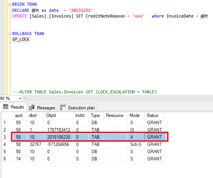
The red box defines an exclusive lock that ensures that multiple updates cannot be made to the same resource at the same time. It occurs in the Invoices table.
Now, we will set the escalation mode for the Sales.Invoices table to automate it and re-run the query.
ALTER TABLE Sales.Invoices SET (LOCK_ESCALATION = AUTO)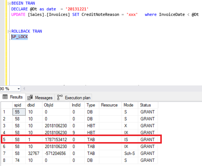
Now, the red box defines the indent exclusive lock that protects requested or acquired exclusive locks on some resources lower in the hierarchy. Shortly, this lock level allows us to update or delete other partition of tables. That means that we can start another update or insert other partition of the table.
In previous posts, we also explored the issue of switching between table partitioning and provided the walkthrough. This information may be of help for you if you deal with these cases. Refer to the article for more information.