Using Indexes in SQL Server Memory-Optimized Tables

Introduction

In this article, we will discuss how different types of indexes in SQL Server memory-optimized tables affect performance. We will examine examples of how different index types can affect the performance of memory-optimized tables.

To make the topic discussion easier, we will make use of a rather large example. For the purposes of simplicity, this example will feature different replicas of a single table, against which we will run different queries. These replicas will use different indexes, or no indexes at all (except, of course, the primary keys – PKs).

Note, that the actual purpose of this article is not to compare performance between disk-based and memory-optimized tables in SQL Server per se. Its purpose is to examine how indexes affect performance in memory-optimized tables. However, in order to have a full picture of the experiments, timings are also provided for the corresponding disk-based table queries and the speedups are calculated using the most optimal configuration of disk-based tables as baselines.

Scenario

Sample data for our scenario is based on a single table defined as the following:

Listing 1: Sample Data Source Table.

The table above was populated with sample data and will act as the data source for the rest of the tables.

So, based on the above table, we create the following 9 table variations and populate them with the same sample data:

• 3 disk-based tables:
  • d_tblSample1
    • Clustered index on the “id” column – primary key (PK)
  • d_tblSample2
    • Clustered index on the “id” column (PK)
    • Non-clustered index on the “countryCode” column
  • d_tblSample3
    • Clustered index on the “id” column (PK)
    • Non-clustered indexes on the “regDate” column
    • Non-clustered indexes on the “countryCode” column
• 3 memory-optimized tables (set 1: Hash indexes):
  • m1_tblSample1
    • Non-clustered hash index on the “id” column – primary key (PK)
  • m1_tblSample2
    • Non-clustered hash index on the “id” column (PK)
    • Hash index on the “countryCode” column
  • m1_tblSample3
    • • Non-clustered hash index on the “id” column (PK)
      • Hash index on the “regDate” column
      • Hash index on the “countryCode” column
  • 3 memory-optimized tables (set 2: Non-Clustered indexes):
    • m2_tblSample1
      • Non-clustered index on the “id” column – primary key (PK)
    • m2_tblSample2
      • Non-clustered index on the “id” column (PK)
      • Non-clustered index on the “countryCode” column
    • m2_tblSample3
      • Non-clustered index on the “id” column (PK)
      • Non-clustered index on the “regDate” column
      • Non-clustered index on the “countryCode” column

In the below listings, you can find the definitions for the above tables.

The scenario logic is that we perform different database operations against variations of the same table (but with different indexes), and observe how performance is affected in each case.

Definitions

Disk-Based Tables

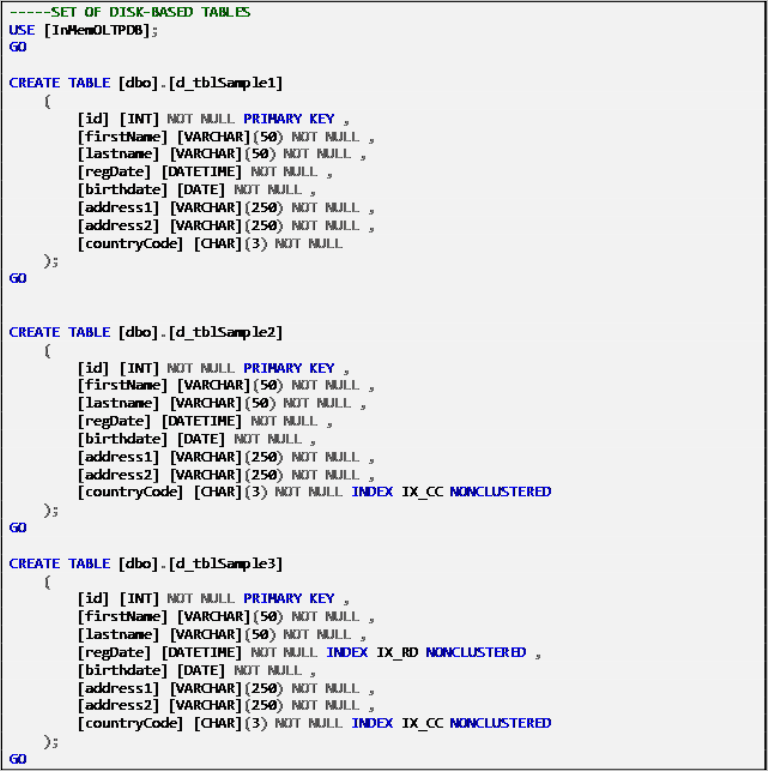
Listing 2: Disk-Based Tables Definition.

Memory-Optimized Tables (Set 1: Hash Indexes)

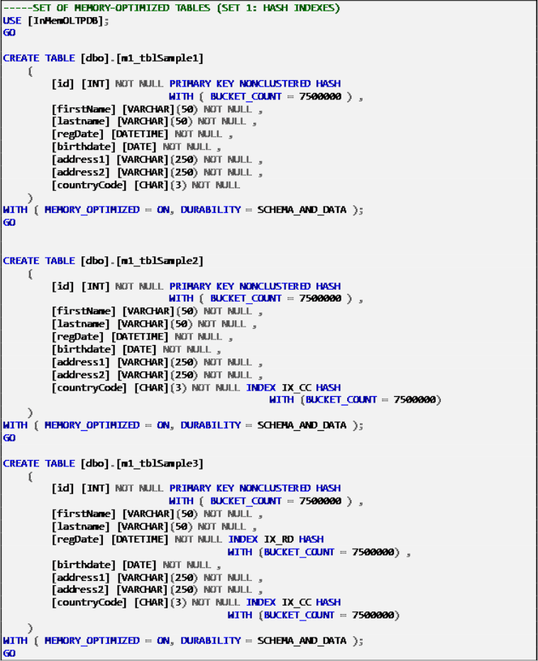
Listing 3: Memory-Optimized Tables – Set 1 (Hash Indexes).

Memory-Optimized Tables (Set 2: Non-Clustered Indexes)

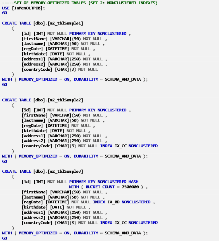
Listing 4: Memory-Optimized Tables – Set 2 (Non-Clustered Indexes).

Then, we populate all the above tables with the same sample data, which is in total 5 million records in each table.

Here’s the output of the count command for each set of tables:

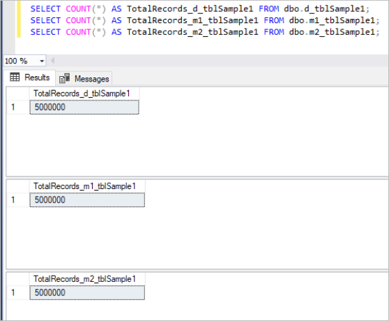
Figure 1: Total Number of Records for First Set of Tables.

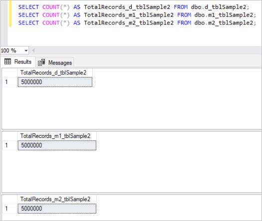
Figure 2: Total Number of Records for Second Set of Tables.

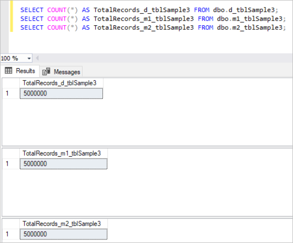
Figure 3: Total Number of Records for Third Set of Tables.

Queries and Scenario Executions

Now, we are going to run a set of queries against the above tables and see how each table performs.

These queries perform the following operations:

• Query 1: Aggregation (GROUP BY)
• Query 2: Index seek on equality predicates
• Query 3: Index seek on equality and inequality predicates

The plan is to execute the queries as per below:

Query 1 – Execution against the following tables:

• d_tblSample3
• m1_tblSample3
• m2_tblSample3
• m1_tblSample1 (no index on target columns)
• m2_tblSample1 (no index on target columns)

Query 2 – Execution against the following tables:

• d_tblSample2
• m1_tblSample2
• m2_tblSample2
• m1_tblSample1 (no index on target columns)
• m2_tblSample1 (no index on target columns)

Query 3 – Execution against the following tables:

• d_tblSample3
• m1_tblSample3
• m2_tblSample3
• m1_tblSample1 (no index on target columns)
• m2_tblSample1 (no index on target columns)

Note: Even though the definition for the d_tblSample1 disk-based table is included in the above table definitions, it is not used in the queries provided in this article. The reason is that, in each scenario, the most optimal possible configuration for the disk-based table is used, as we want our baseline to be as fast as possible when we compare it with the performance of memory-optimized tables. To this end, the d_tblSample1 table  is just presented for informational purposes.

Below you can find the T-SQL scripts for the three queries along with the execution time measuring mechanisms.

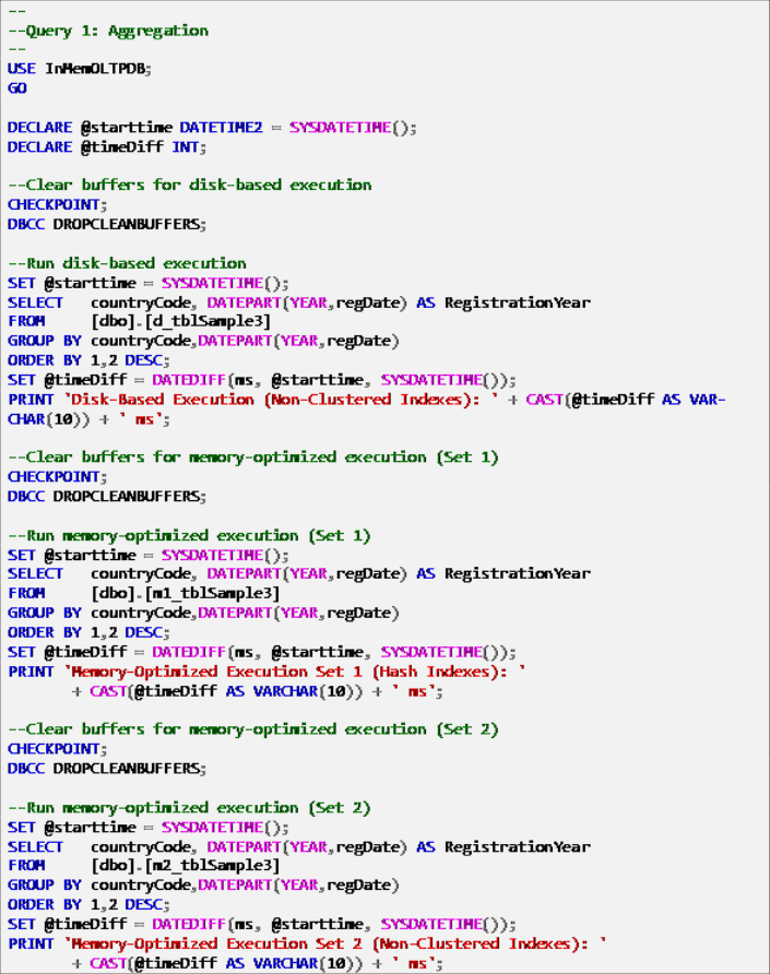
Listing 5: Query 1 – Aggregation (with indexes).

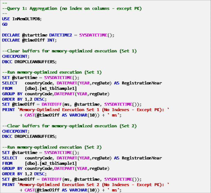
Listing 6: Query 1 – Aggregation (with no indexes – Except Primary Key).

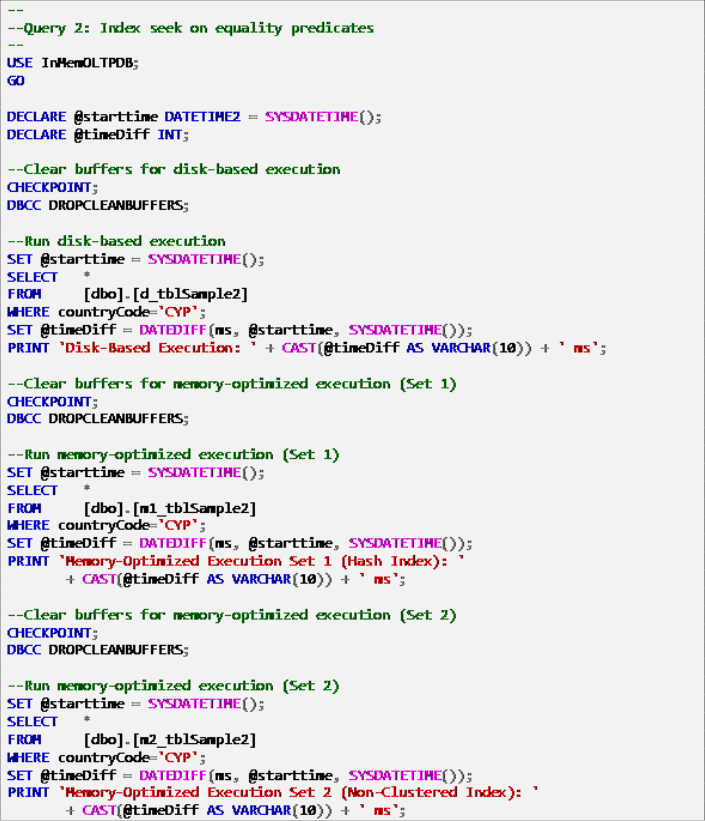
Listing 7: Query 2 – Index Seek on Equality Predicates (with indexes).

Listing 8: Query 2 – Index Seek on Equality Predicates (with no indexes – except Primary Key).

Listing 9: Query 3 – Index Seek on Equality and Inequality Predicates (with indexes).

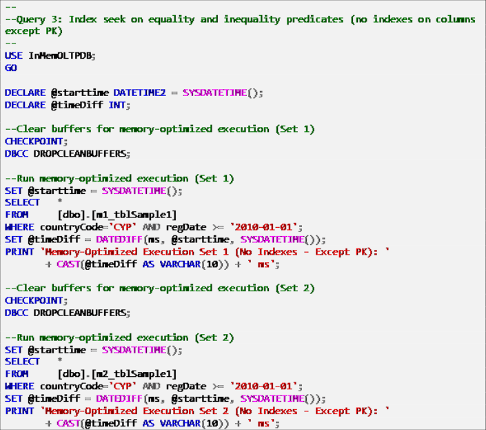
Listing 10: Query 3 – Index Seek on Equality and Inequality Predicates (with no indexes – Except Primary Key).

The screenshots below show the output of each query execution:

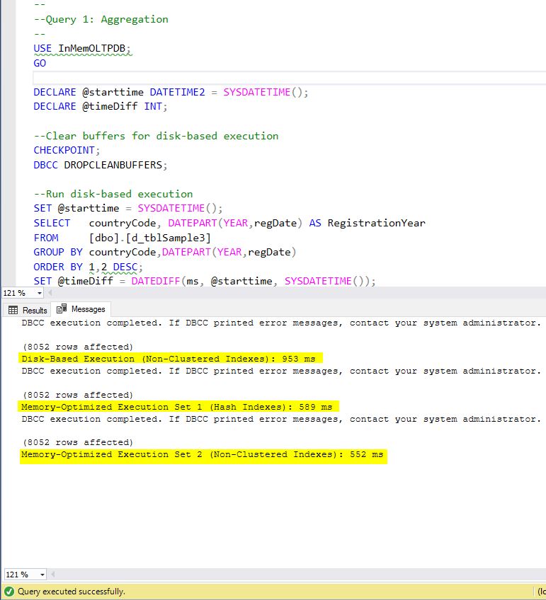
Figure 4: Query 1 Execution Time (with indexes).

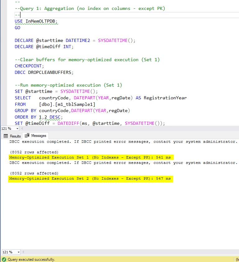
Figure 5: Query 1 Execution Time (with no indexes – except PK).

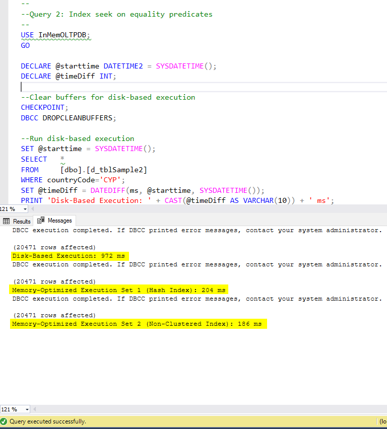
Figure 6: Query 2 Execution Time (with indexes).

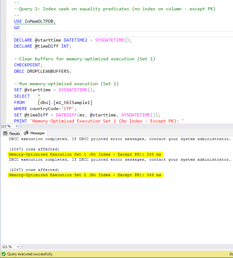
Figure 7: Query 2 Execution Time (with no indexes – except PK).

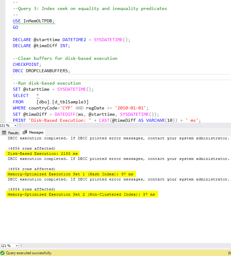
Figure 8: Query 3 Execution Time (with indexes).

Figure 9: Query 3 Execution Time (with no indexes – except PK).

Now, let’s summarize the results obtained above. The following table displays the measured execution times for all the above queries and table/index combinations.

Table 1: Summary of Execution Times (ms) for all Queries.

Discussion

If we examine the execution results summarized in the table above, we can reach certain conclusions. Let’s plot each query result into a graph. The graphs below illustrate the execution times, as well as the speedup of the memory-optimized tables over the disk-based tables.

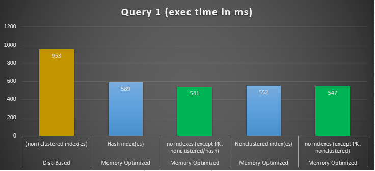
Figure 10: Query 1 Execution Times Comparison.

Figure 11: Query 1 Speedup Comparison.

Regarding Query 1, which was a GROUP BY aggregation, we can see that both versions (indexes vs no indexes) of memory-optimized tables, perform almost the same having a speedup over the disk-based table (enabled with indexes) between 1.62 and 1.76 times faster.

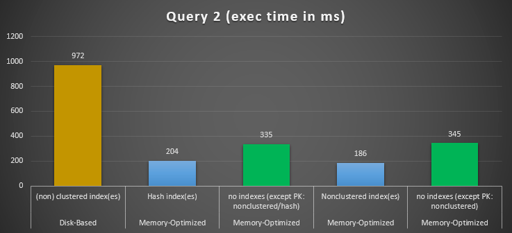
Figure 12: Query 2 Execution Times Comparison.

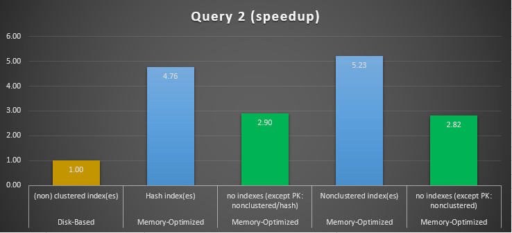
Figure 13: Query 2 Speedup Comparison.

Regarding Query 2, which involved an index seek on equality predicates, we can see that the memory-optimized tables with indexes performed much better than the memory-optimized tables with no indexes. Moreover, we observe that the memory-optimized table with non-clustered index in the column used as a predicate performed better than the one with the hash index.

So, for query 2, the winner is the memory-optimized table with the non-clustered index, having an overall speedup of 5.23 times faster over disk-based execution.

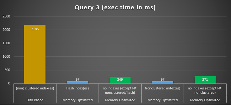
Figure 14: Query 3 Execution Times Comparison.

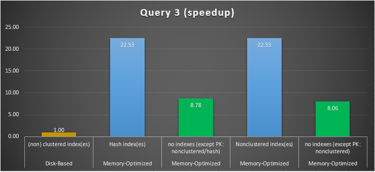
Figure 15: Query 3 Speedup Comparison.

Regarding Query 3, which involved an index seek on equality and inequality predicates combined, we can see that the memory-optimized tables with indexes, performed a way better than the memory-optimized tables with no indexes. Moreover, we observe that the memory-optimized table with non-clustered index in the column used as a predicate performed the same as the one with the hash index.

To this end, we can see that both memory-optimized tables which make use of indexes in the columns used as predicates, performed faster than the ones with no indexes and achieved a speedup of 22.53 times faster over disk-based execution.

Conclusion

In this article, we examined the usage of indexes in memory-optimized tables in SQL Server. We used as a baseline for each query, the best possible disk-based table configuration, and then we compared the performance of three queries against the disk-based tables, and 4 variations of memory-optimized tables. Two out of four memory-optimized tables used indexes (hash/non-clustered) and the other two used no indexes, except the ones used for the primary keys.

The overall conclusion is that you always need to examine how indexes affect performance, not only for memory-optimized tables but also for disk-based ones, and whenever you identify that they improve performance, to use them. The findings of this article’s examples, show that if you make use of the proper indexes in memory-optimized tables, you can achieve much better performance for queries similar to the ones used in this article when compared to just using memory-optimized tables without indexes.

References and Further Reading:

1. Microsoft Docs: Memory-Optimized Tables
2. Microsoft Docs: Guidelines for Using Indexes on Memory-Optimized Tables
3. Microsoft Docs: Indexes on Memory-Optimized Tables

Useful tool:

dbForge Index Manager – handy SSMS add-in for analyzing the status of SQL indexes and fixing issues with index fragmentation.