Analytic Functions in SQL Server

Aggregate and Analytic functions in SQL Server operate on a set of rows. However, unlike such aggregate functions as sum, count and average that return scalar values, analytic functions return a group of rows that can be further analyzed. In this article, we will see some of the most commonly used analytic functions in SQL server. We will be discussing the following functions:

• CUME_DIST
• FIRST_VALUE
• LAST_VALUE
• LEAD
• LAG

Creating Dummy Data

Let’s prepare some dummy data that we will be using to execute our queries.
Execute the following script:

CREATE DATABASE Showroom

Use Showroom
CREATE TABLE Car
(
CarId int identity(1,1) primary key,
Name varchar(100),
Make varchar(100),
Model int ,
Price int ,
Type varchar(20)
)

insert into Car( Name, Make, Model , Price, Type)
VALUES ('Corrolla','Toyota',2015, 20000,'Sedan'),
('Civic','Honda',2018, 25000,'Sedan'),
('Passo','Toyota',2012, 18000,'Hatchback'),
('Land Cruiser','Toyota',2017, 40000,'SUV'),
('Corrolla','Toyota',2011, 17000,'Sedan'),
('Vitz','Toyota',2014, 15000,'Hatchback'),
('Accord','Honda',2018, 28000,'Sedan'),
('7500','BMW',2015, 50000,'Sedan'),
('Parado','Toyota',2011, 25000,'SUV'),
('C200','Mercedez',2010, 26000,'Sedan'),
('Corrolla','Toyota',2014, 19000,'Sedan'),
('Civic','Honda',2015, 20000,'Sedan')

In the script above, we create Showroom database with one table Car. The Car table has five attributes. CarId, Name, Make, Model, Price and Type. Next, we added 12 dummy records in the Car table.

Let’s now see each of the analytic function in detail:

CUME_DIST

As per SQL Server Official Documentation, the cume_dist function is used to find the cumulative distribution of a value among the group of values. Simply speaking, the cumulative distribution value for a row can be calculated by dividing the rank of the row (as defined by the ORDER BY clause) by the total number of rows in the group. It is best explained with an example.

Execute the following script:

Use Showroom
SELECT Name,Make,Model, Price, Type,
CUME_DIST() OVER(ORDER BY Price) as PriceDistribution
FROM Car

To execute the cume_dist function, the OVER clause is mandatory. Inside the OVER clause the ORDER BY clause is used to sort the data. In the script above, we SELECT the Name, Make, Model, Price and the cumulative distribution with respect to the ascending order of the Price.

The output of the script above looks like this:

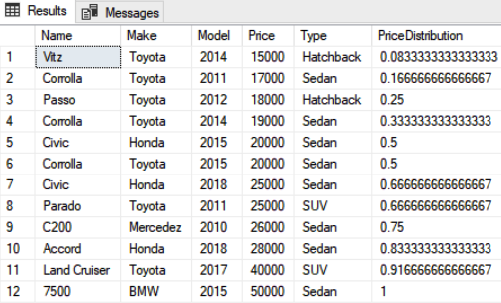
The values for the cumulative distributions are mentioned in column “PriceDistribution”. You can see that the value for row 12 is 1. This is because at row 12, all the other rows have values less or equal to 12. Therefore, 12/12 =1. Similarly, look at the record 9 where the value is 0.75. This is because at row 9, at least 9 or less rows have price value less than the current row, therefore 9/12 is 0.75.

Similarly, the cume_dist function can also be used with partitioned data. Look at the following example:

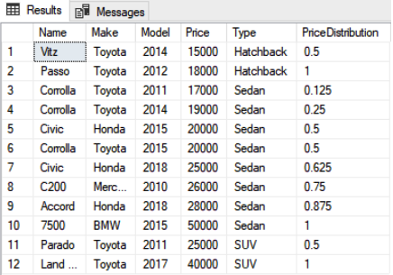
Use Showroom
SELECT Name,Make,Model, Price, Type,
CUME_DIST() OVER (PARTITION BY Type ORDER BY Price) as PriceDistribution
FROM Car

The above script returns the cumulative distribution of the rows partitioned by the Type and sorted by the price. The script returns the following value:

FIRST_VALUE

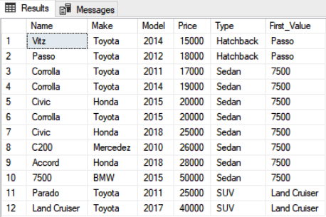
The first_value function retrieves the first value from the specified column for the records that have been sorted using the ORDER BY clause. Look at the following script:

Use Showroom
SELECT Name, Make, Model, Price, Type,
FIRST_VALUE(Name) OVER(ORDER BY Price) as First_Value
FROM Car c

The output of the script above looks like this:

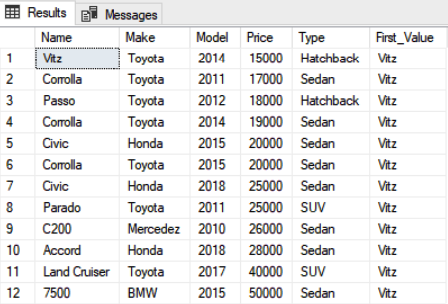
Since the car “Vitz” is the cheapest car or the first value in the sorted vehicle list, you can see this value in the “First_Value” column.

You can also use the first_value function with the PARTITION BY clause. You will see the first value from each partition in the output. Execute the following script:

Use Showroom
SELECT Name, Make, Model, Price, Type,
FIRST_VALUE(Name) OVER(PARTITION BY Type ORDER BY Price) as First_Value
FROM Car c

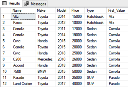
Now you can see the least expensive car in front of each partition. For instance, among the hatchbacks, Toyota Vitz is the least expensive whereas among sedans, Toyota Corolla 2011 is the least expensive model.

LAST_VALUE

The last_value function is the reverse of the first value function and returns the last value for specific column from the ordered sequence. Execute the following script:

Use Showroom
SELECT Name, Make, Model, Price, Type,
FIRST_VALUE(Name) OVER(PARTITION BY Type ORDER BY Price) as First_Value
FROM Car c

The output looks like this:

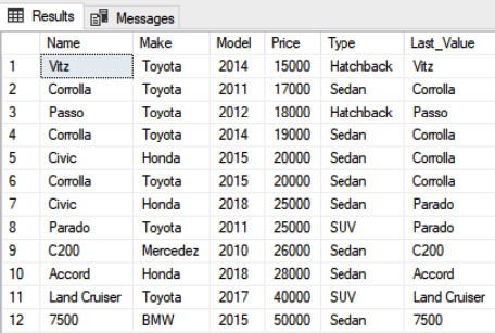
You can see that the output is not what we expected. The last value in the sorted price list is the 50,000 that belongs to BMW 7500, however we see different values in the Last_Value column.

The reason behind this behavior is that by default the range values used for ROWS in the Last_Value function are BETWEEN UNBOUNDED PRECEDING and CURRENT ROW. It means that the last value is selected from the start of the records and the current row. So in the first iteration, only the first row is taken into account and, hence, its name is added to the Last_Value column. Similarly, in the second iteration, the first two rows are evaluated and since the second row contains the last value, it has been added to the Last_Value column.

A solution to this problem is to specify UNBOUNDED PRECEDING AND UNBOUNDED FOLLOWING as the range for ROW. Look at the following script:

Use Showroom
SELECT Name, Make, Model, Price, Type,
LAST_VALUE(Name) OVER(ORDER BY Price ROWS BETWEEN UNBOUNDED PRECEDING AND UNBOUNDED FOLLOWING) as Last_Value
FROM Car c

The output of the script above looks like this:

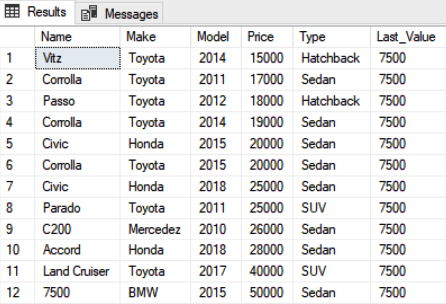
Now, you can see BMW 7500 series as the last value.

Like First_Value function, the Last_Value function can also be used with the PARTITION BY clause. The following script does that:

Use Showroom
SELECT Name, Make, Model, Price, Type,
LAST_VALUE(Name) OVER(PARTITION BY Type ORDER BY Price ROWS BETWEEN UNBOUNDED PRECEDING AND UNBOUNDED FOLLOWING) as First_Value
FROM Car c

The output of the script above looks like this:

LEAD

The lead function is used to retrieve the values from next N rows. The column from which the value is to be fetched and the number of rows to be offset is specified inside the lead function. Look at the following script:

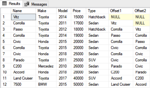
Use Showroom
SELECT Name, Make, Model, Price, Type,
LEAD(Name,1) OVER(ORDER BY Price) as Offset1,
LEAD(Name,2) OVER(ORDER BY Price) as Offset2
FROM Car c

In the script above, we specified it for each record by retrieving the values from the Name column of the next 1 and then 2 records. Here is the output:

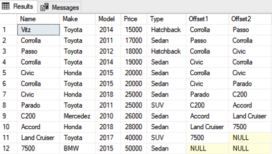
Here you can see that for the first row in the Offset1 column, you can see “Corolla” as the name of the car model in the second row. Similarly, for the Offset2 column in the first row, you can see “Passo” as the name of the third car. Finally, if you see the last row, since there is no row after that, both the Offset1 and Offset2 columns contain NULL.

LAG

The lag function is reverse of the lead function and is used to retrieve the values from previous N rows. The column from which the value is to be fetched and the number of rows to be offset is specified inside the lag function

Use Showroom
SELECT Name, Make, Model, Price, Type,
LAG(Name,1) OVER(ORDER BY Price) as Offset1,
LAG(Name,2) OVER(ORDER BY Price) as Offset2
FROM Car c

In the script above, we specified that for each record by retrieving the values from the Name column of the previous 1 and 2 records. Here is the output:

Conclusion

Analytic functions were introduced in SQL Server 2012. They are used to perform operations on a set of rows. In this article, we presented the most commonly used analytic functions in SQL Server as well we their application.