Everything you should know about SQL Server JOINS

The focus of this article is going to be on utilizing JOINs. We will start off by talking a bit about how JOINs are going to happen and why you need to JOIN data. Then we will take a look at the JOIN types that we have available to us and how to use them.

JOIN BASICS

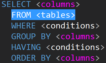
JOINs in TSQL are typically going to be done on the FROM line.

Before we are getting to anything else, the real big question becomes — “Why do we have to do JOINs, and how are we actually going to perform our JOINs?”

As it turns out, every database that we ever work with is going to have its data split up into multiple tables. There are many different reasons for this:

• Maintaining data integrity
• Saving stored space
• Editing data faster
• Making queries more flexible

Thus, every database that you are going to be working with is going to need that data to be joined together in order for it to actually make sense.

For example, you have separate tables for orders and for customers. The question that becomes — “How do we actually connect all data together?” That is exactly what JOINs are going to do.

HOW JOINs WORK

Imagine the case, when we have two separate tables and those tables are going to be brought together by creating a seam.

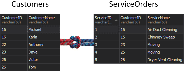
What is going to happen with the seam, if we get one column from each table that is going to be used for matching, and that is going to determine what rows are or are not going to be returned? For example, we have Customers on the left and ServiceOrders on the right. If we want to get all the customers and their orders, we need to JOIN these two tables together. For this, we need to choose one column that will act as a seam, and obviously, of course, the column we are going to use is CustomerID.

By the way, the CustomerID is known as a Primary Key for the left table, which uniquely identifies every single row inside the Customers table.

In the ServiceOrders table, we also have the CustomerID column, which is known as a Foreign Key. A foreign key is simply a column that is designed to point to another table. In our case, it is pointing back to the Customers table. Therefore, that is how we are going to bring all of that data together by providing that seam.

In these tables, we have the following matchings: 2 orders for 15 and 1 order for 23, 25, and 26. 16 and 22 are left out.

One big thing to note here is that we can JOIN multiple tables. In fact, it is quite common to JOIN multiple tables together, in order to get any form of information. If you take a look at the most common database, you may have to JOIN together four, five, six and more tables just to get the information you are looking for. Having a database diagram is going to be helpful.

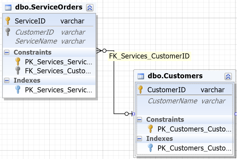
To help you out in most database environments you will notice that the columns designed to be JOINed have the same name.

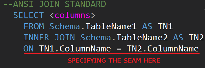
JOIN SYNTAX

The third revision of the SQL database query language (SQL-92) regulates the JOIN syntax:

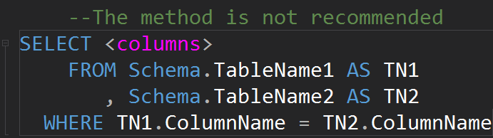
It is possible to do JOINs on WHERE line:

A relation usually has a simple graphical interpretation in the form of a table.

Best Practices and Conventions

1. Alias table names.
2. Use two-part naming for columns
3. Place each JOIN on a separate line
4. Place tables in a logical order

JOIN TYPES

SQL Server provides the following types of JOINs:

• INNER JOIN
• OUTER JOIN
• SELF JOIN
• CROSS JOIN

For more information on the topic, feel free to check this article about the types of joins in SQL Server and learn how easy it is to write such queries with the help of SQL Complete.

INNER JOIN

The first type of JOINs that we may want to execute is the INNER JOIN. Usually, authors refer to this type of SQL Server JOINs as a regular or simple JOIN. They just omit the INNER prefix. This type of JOIN combines two tables together and only returns rows from both sides that match.

We do not see Klara and Anthony here because their CustomerID does not match in both tables. I want to also highlight the fact that the JOIN operation returns a customer each time that it matches the order. There are two orders for Michael and one order for Dave, Victor, and Tom each.

Summary:

• INNER JOIN returns rows only when there is at least one row in both tables that matches the JOIN condition.
• INNER JOIN eliminates the rows that do not match with a row from the other table

OUTER JOIN

Outer JOINs are different because they return rows from tables or views even if they do not match. This type of JOIN is useful if you need to retrieve all customers who have never placed an order. Or, for example, if you are looking for a product that has never been ordered.

The way that we do our OUTER JOINs is by indicating LEFT or RIGHT, or FULL.

There are no differences between the following clauses:

• LEFT OUTER JOIN = LEFT JOIN
• RIGHT OUTER JOIN = RIGHT JOIN
• FULL OUTER JOIN = FULL JOIN

However, I would recommend writing the complete clause because it makes the code more readable.

Using LEFT OUTER JOIN

There is no difference between LEFT or RIGHT except the fact that we just point the table that we want to get the extra rows from.  In the following example, we listed customers and their orders. We utilize the LEFT to get all customers who have never placed orders. We ask SQL Server to get us extra rows from the left table.

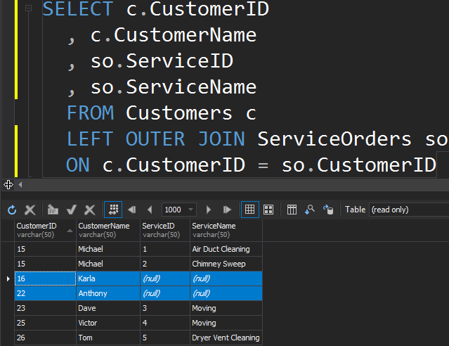
Note that Karla and Anthony have not placed any orders and as a result, we get NULL values for the ServiceName and ServiceID. SQL Server doesn’t know what to place in there, and it places NULLs.

Using RIGHT OUTER JOIN

To get the less popular service from the ServiceOrders table, we need to use the RIGHT direction.

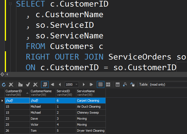
We see that in this case, SQL Server returned extra rows from the right table, and the Carpet Cleaning service has never been ordered.

Using FULL OUTER JOIN

This type of JOIN allows you to get the non-matching information by including non-matching rows from both tables.

This may also be useful if you need to do a data cleanup.

Summary:

FULL OUTER JOIN

• Returns rows from both tables even if they do not match the JOIN statement

LEFT or RIGHT

• No difference except in the order of tables in FROM clause
• Direction points at a table to retrieve non-matching rows from

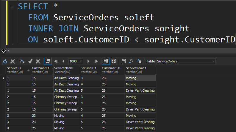
SELF JOIN

The next type of JOINs that we have is SELF JOIN. This is probably the second least common type of JOIN that you are ever going to execute. A SELF JOIN is when you are joining a table onto itself. Generally speaking, this is a sign of poor design. To use the same table twice in a single query, the table must be aliased. The alias helps the query processor identify whether columns should present data from the right or left side. Additionally, you need to eliminate rows marching themselves. This is typically done with a non-equi join.

Summary:

• JOINs a table to itself
• Generally a sign of poor design and normalization
• Tables must be aliased
• Need to filter rows matching themselves

CROSS JOINS

This type of JOINs does not have the ON statement. Every single row from each table is going to match. This is also known as Cartesian Product (in case a CROSS JOIN does not have a WHERE clause). You will hardly use this JOIN type in real-world scenarios, however, it is a good way to generate test data.

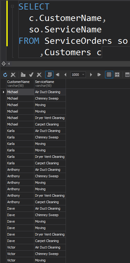
The result is a dataset, where the number of rows in the left table multiplied by the number of rows in the right table. Eventually, we see that every single customer matches every single service.

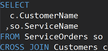
We get the same result when using the CROSS JOIN clause explicitly.

Summary:

• All rows match from each table
• No ON statement
• Can be used to generate test data

JOIN ALGORITHMS

In the first part of the article, we have discussed logical JOIN operators SQL Server uses while query parsing and binding. They are:

• INNER JOIN
• OUTER JOIN
• CROSS JOIN

The logical operators are conceptual and they differ from the physical JOINs. Otherwise speaking, logical JOINs do not actually join particular table columns. A single logical JOIN may correspond to many physical JOINs.  SQL Server replaces logical JOINs to physical JOINs during optimization. SQL Server has the following physical JOIN operators:

• NESTED LOOP
• MERGE
• HASH

A user does not write or use these types of JOINS. They are part of the SQL Server engine and SQL Server uses them internally to implement logical JOINs. When you explore the execution plan, you may note that SQL Server replaces logical JOIN operators with one of three physical operators.

Nested Loop Join

Let’s start from the simplest operator, which is Nested Loop. The algorithm compares every single row of one table (outer table) to each row of the other table (inner table) looking for rows that meet the JOIN predicate.

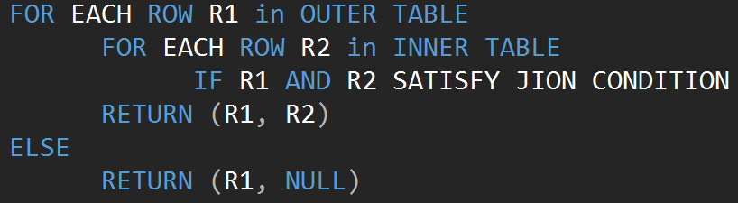
The following pseudo-code describes the inner nested join loop algorithm:

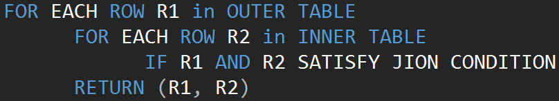
The following pseudo-code describes the outer nested join loop algorithm:

The size of the input directly affects the algorithm cost. The input grows the cost grows also. This type of JOIN algorithm is efficient in case of small input. SQL Server estimates a JOIN predicate for every row in both inputs.

Consider the following query as an example, which gets customers and their orders.

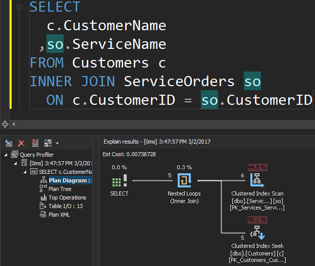
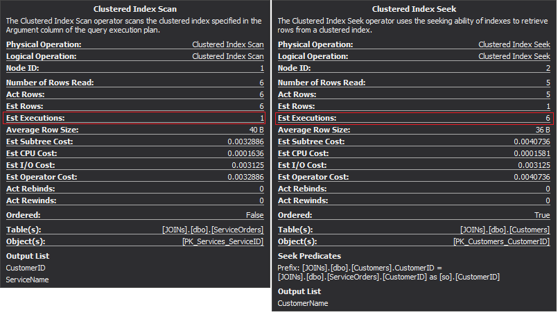
The Clustered Index Scan operator is the outer input and the Clustered Index Seek is the inner input. The Nested Loop operator actually finds matching. The operator looks for each record in the outer input and finds matching rows in the inner input. SQL Server executes the Clustered Index Scan operation (outer input) only once to get all relevant records. Clustered Index Seek is executed for each record from the outer input. To confirm this, navigate the cursor to the operator icon and examine the tooltip.

Let’s talk about the complexity. Suppose N is the row number for the outer output. M is the total row number in the SalesOrders table. Thus, the complexity of the query is O(NLogM) where LogM is the complexity of each seek in the inner input. The optimizer will select this operator every time when the outer input is small and the inner input contains an index in the column that acts as the seam. Therefore, indexes and statistics are essential for this JOIN type, otherwise SQL Server may accidentally think that there are not so many rows in one of the inputs. It is better to perform one table scan rather than performing Index Seek 100K times. Especially when the inner input size is more than 100K.

Summary:

Nested Loops

• Complexity: O(NlogM)
• Applied usually when one table is small
• The larger table contains an index which allows seeking it using the join key

Merge Join

Some developers do not completely understand Hash and Merge JOINs and frequently associate them with poor performing queries.

As opposed to Nested Loop that accepts any JOIN predicate, the Merge Join requires at least one equi join. Additionally, both inputs must be sorted on the JOIN keys.

The pseudo-code for the MERGE JOIN algorithm:

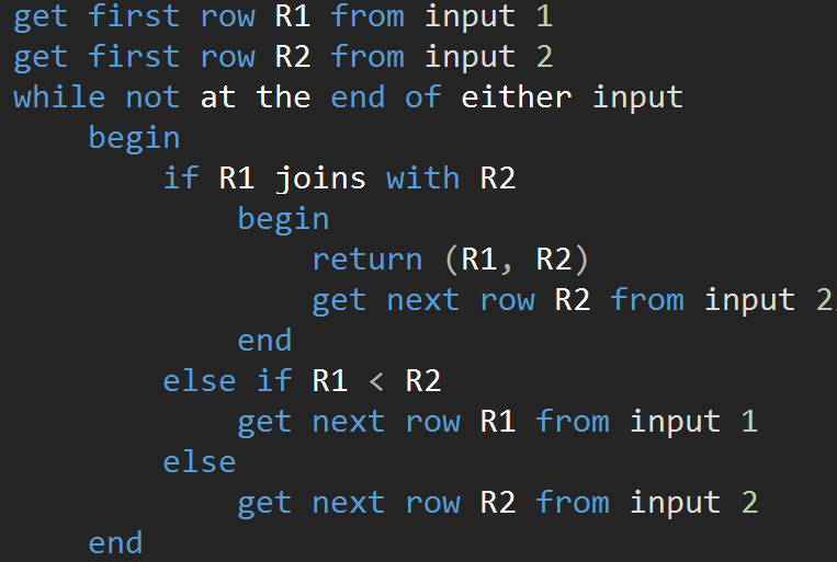
The algorithm compares two sorted inputs. One row at a time. In case there is an equality between two rows, the algorithm outputs join rows and continue. If not, the algorithm discards the lesser of the two inputs and continue. Unlike the Nested Loop, the cost here is proportional to the sum of the number of input rows. In terms of complexity – O(N+M). Therefore, this type of JOINs is often better for large inputs.

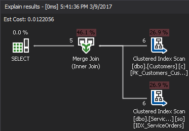
The following animation demonstrates how the MERGE JOIN algorithm actually joins table rows.

Summary

• Complexity: O(N+M)
• Both inputs must be sorted on the join key
• An equality operator is used
• Excellent for large tables

Hash Join

Hash Join is well suited for large tables without usable index. On the first step – build phase the algorithm creates an in-memory hash index on the left-side input. The second step is called the probe phase. The algorithm goes through the right-side input and finds matches using the index created during the build phase. If say to truth, it is not a good sign when the optimizer chooses this type of JOIN algorithm.

There are two important concepts underlying this type of JOINs: Hash function and Hash Table.

A hash function is any function that may be used to map data of variable size to data of fixed size.

A hash table is a data structure used to implement an associative array, a structure that can map keys to values. A hash table uses a hash function to compute an index into an array of buckets or slots, from which the desired value can be found.

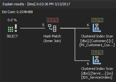
Based on the available statistics, SQL Server chooses the smallest input as the build input and uses it to build a hash table in memory. If there is not enough memory, SQL Server uses physical disk space in TempDB. Once the hash table is created, SQL Server gets the data from the probe input (larger table) and compares it to the hash table using a hash match function. As a result, it returns matched rows.

If we look at the execution plan, the right top element is the build input, and the right bottom element is the probe input. In case both inputs are extremely large, the cost is too high.

To estimate the complexity, assume the following:

h_c – complexity of the hash table creation

h_m – complexity of the hash match function

N – smaller table

M – larger table

J – complexity addition for the dynamic calculation and creation of the hash function

The complexity will be: O(N*h_c + M*h_m + J)

The optimizer uses statistics to determine value cardinality. Then it dynamically creates a hash function that divides data into many buckets with equal sizes. It is often difficult to estimate the complexity of the hash table creation process, as well as the complexity of each hash match due to dynamic nature. The execution plan may even show incorrect estimations because optimizer performs all these dynamic operations during the execution time. In some cases, the execution plan may show that Nested Loop is more expensive than Hash Join, but in fact, the Hash Join executes slower due to the incorrect cost estimation.

Summary

• Complexity: O(N*h_c+M*h_m+J)
• Last-resort join type
• Uses a hash table and a dynamic hash match function to match rows

Useful products:

SQL Complete – write, beautify, refactor your code easily and boost your productivity.