
Grouping is an important feature that helps organize and arrange data. There are a lot of ways to do it, and one of the most effective methods is the SQL GROUP BY clause.
You can use SQL GROUP BY to divide rows in results into groups with an aggregate function. It sounds easy to sum, average, or count records with it.
But are you doing it right?
“Right” can be subjective. When it runs without critical errors with a correct output, it’s considered to be fine. However, it needs to be quick too.
In this article, speed will also be considered. You will see much query analysis using logical reads and execution plans in all the points.
Let’s begin.
GROUP BY Clause
In the realm of SQL, the GROUP BY clause plays a pivotal role in organizing unsorted, raw data into meaningful groups. It is an essential tool for anyone dealing with large databases, as it allows for the aggregation of data based on specified columns.
Definition and Purpose of the GROUP BY Clause
The GROUP BY clause is a SQL command used primarily with the SELECT statement to arrange identical data into groups. This clause follows the WHERE clause in a SELECT statement and precedes the ORDER BY clause. The primary purpose of the GROUP BY clause is to provide a means to aggregate data into groups, which can then be subjected to various aggregate functions like COUNT, SUM, AVG, MAX, or MIN.
In essence, the GROUP BY clause turns a detailed table of data into a small, organized table with grouped and summarized data. This is particularly useful when dealing with large databases where you need to summarize data in a meaningful way. For instance, you might want to know the total sales for each region in your company, or perhaps the average grade for students in each class at a school. The GROUP BY clause makes such tasks straightforward and efficient.
Basic Syntax of the GROUP BY Clause
The basic syntax of the GROUP BY clause is as follows:
SELECT column1, column2, ..., aggregate_function(column)
FROM table
WHERE conditions
GROUP BY column1, column2, ...;
In this syntax, column1, column2, ... are the columns that you want to group by. The aggregate_function(column) could be any function like SUM, COUNT, AVG, MAX, or MIN that will perform an operation on the grouped data. The WHERE clause is optional and can be used to filter rows before they are grouped.
Here’s a simple example:
SELECT Country, COUNT(CustomerID)
FROM Customers
GROUP BY Country;
In this query, the GROUP BY clause groups the customers by country, and the COUNT(CustomerID) function returns the number of customers in each country.
Understanding the GROUP BY clause is fundamental to mastering SQL, as it allows for powerful data analysis and manipulation. In the following sections, we will delve deeper into how to use this clause effectively with various SQL commands and functions.
Example 1: SQL GROUP BY with WHERE or HAVING Clauses
If you’re confused about when to use WHERE and HAVING, this one is for you. Because depending on the condition you provide, both may give the same result.
But they’re different.
HAVING filters the groups using the columns in the SQL GROUP BY clause. WHERE filters the rows before grouping and aggregations occur. So, if you filter using the HAVING clause, grouping occurs for all rows returned.
And that’s bad.
Why? The short answer is: it’s slow. Let’s prove this with 2 queries. Check out the code below. Before running it in SQL Server Management Studio, press Ctrl-M first.
Using WHERE Clause
SET STATISTICS IO ON
GO

SELECT
 MONTH(soh.OrderDate) AS OrderMonth
,YEAR(soh.OrderDate) AS OrderYear
,p.Name AS Product
,SUM(sod.LineTotal) AS ProductSales
FROM Sales.SalesOrderHeader soh
INNER JOIN Sales.SalesOrderDetail sod ON soh.SalesOrderID = sod.SalesOrderID
INNER join Production.Product p ON sod.ProductID = p.ProductID
WHERE soh.OrderDate BETWEEN '01/01/2012' AND '12/31/2012'
GROUP BY p.Name, YEAR(soh.OrderDate), MONTH(soh.OrderDate)
ORDER BY Product, OrderYear, OrderMonth;

SET STATISTICS IO OFF
GO
Using HAVING Clause
SET STATISTICS IO ON
GO

SELECT
 MONTH(soh.OrderDate) AS OrderMonth
,YEAR(soh.OrderDate) AS OrderYear
,p.Name AS Product
,SUM(sod.LineTotal) AS ProductSales
FROM Sales.SalesOrderHeader soh
INNER JOIN Sales.SalesOrderDetail sod ON soh.SalesOrderID = sod.SalesOrderID
INNER join Production.Product p ON sod.ProductID = p.ProductID
GROUP BY p.Name, YEAR(soh.OrderDate), MONTH(soh.OrderDate)
HAVING YEAR(soh.OrderDate) = 2012
ORDER BY Product, OrderYear, OrderMonth;

SET STATISTICS IO OFF
GO
WHERE vs HAVING: A Study in SQL Query Performance
The two SELECT statements above will return the same rows. Both are correct in returning product orders by month in the year 2012. But the first SELECT took 136ms. to run on my laptop, while another one took 764ms.!
Why?
Let’s check the logical reads first in Figure 1. The STATISTICS IO returned these results. Then, I pasted it into StatisticsParser.com for the formatted output.
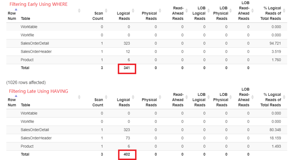
Figure 1. Logical reads of filtering early using WHERE vs. filtering late using HAVING.
Look at the total logical reads of each. To understand these numbers, the more logical reads it took, the slower the query will be. So, it proves that using HAVING is slower, and filtering early with WHERE is faster.
Of course, this does not mean that HAVING is useless. One exception is when using HAVING with an aggregate like HAVING SUM(sod.Linetotal) > 100000. You can combine a WHERE clause and a HAVING clause in one query.
See the execution plan in Figure 2.
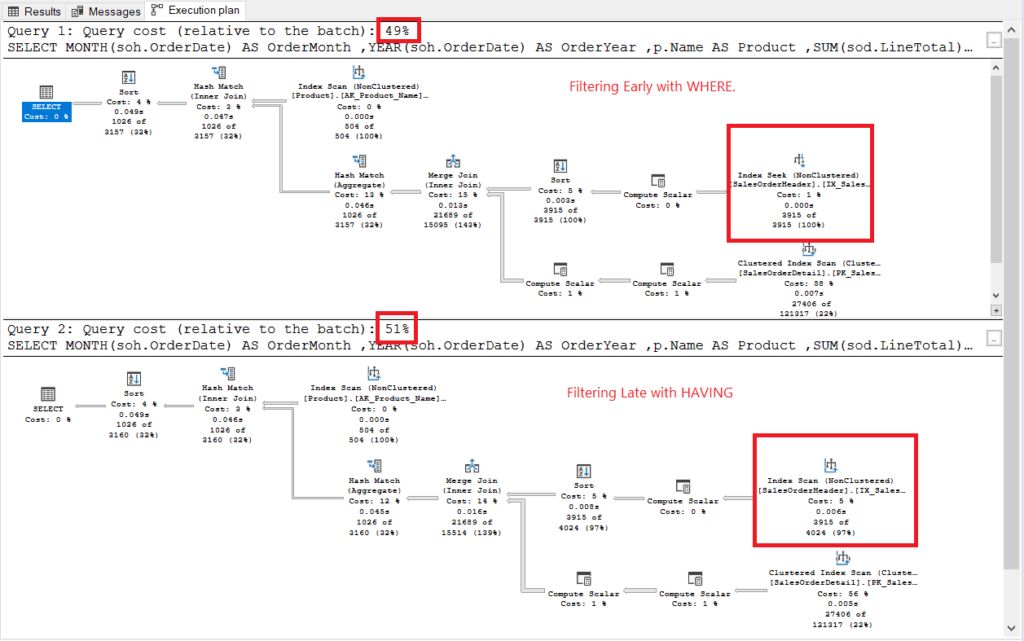
Figure 2. Execution plans of filtering early vs. filtering late.
Both execution plans looked similar except for the ones boxed in red. Filtering early used the Index Seek operator while another one used Index Scan. Seeks are faster than scans in large tables.
Note: Filtering early has less cost than filtering late. So, the bottom line is filtering the rows early can improve the performance.
Example 2: Combining GROUP BY and JOIN in SQL Server
Joining some of the tables you need later can also improve performance.
Let’s say you want to have monthly product sales. You also need to get the product name, number, and subcategory all in the same query. These columns are in another table. And they all need to be added in the GROUP BY clause to have a successful execution. Here’s the code.
SET STATISTICS IO ON
GO

SELECT
 p.Name AS Product
,p.ProductNumber
,ps.Name AS ProductSubcategory
,SUM(sod.LineTotal) AS ProductSales
FROM Sales.SalesOrderHeader soh
INNER JOIN Sales.SalesOrderDetail sod ON soh.SalesOrderID = sod.SalesOrderID
INNER JOIN Production.Product p ON sod.ProductID = p.ProductID
INNER JOIN Production.ProductSubcategory ps ON p.ProductSubcategoryID = ps.ProductSubcategoryID
WHERE soh.OrderDate BETWEEN '01/01/2012' AND '12/31/2012'
GROUP BY p.name, p.ProductNumber, ps.Name
ORDER BY Product

SET STATISTICS IO OFF
GO
This will run fine. But there’s a better, faster way. This won’t require you to add the 3 columns for product name, number, and subcategory in the GROUP BY clause. Though, this will require a bit more keystrokes. Here it is.
SET STATISTICS IO ON
GO

;WITH Orders2012 AS
(
SELECT
 sod.ProductID
,SUM(sod.LineTotal) AS ProductSales
FROM Sales.SalesOrderHeader soh
INNER JOIN Sales.SalesOrderDetail sod ON soh.SalesOrderID = sod.SalesOrderID
WHERE soh.OrderDate BETWEEN '01/01/2012' AND '12/31/2012'
GROUP BY sod.ProductID
)
SELECT
 P.Name AS Product
,P.ProductNumber
,ps.Name AS ProductSubcategory
,o.ProductSales
FROM Orders2012 o
INNER JOIN Production.Product p ON o.ProductID = p.ProductID
INNER JOIN Production.ProductSubcategory ps ON p.ProductSubcategoryID = ps.ProductSubcategoryID
ORDER BY Product;

SET STATISTICS IO OFF
GO
Performance Analysis: JOIN and GROUP BY in SQL Queries
Why is this faster? The joins to Product and ProductSubcategory are done later. Both are not involved in the GROUP BY clause. Let’s prove this by numbers in the STATISTICS IO. See Figure 4.
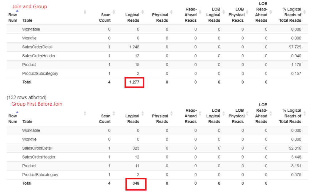
Figure 3. Joining early then grouping consumed more logical reads than doing the joins later.
See those logical reads? The difference is far, and the winner is obvious.
Let’s compare the execution plan of the 2 queries to see the reason behind the numbers above. First, see Figure 4 for the execution plan of the query with all tables joined when grouped.
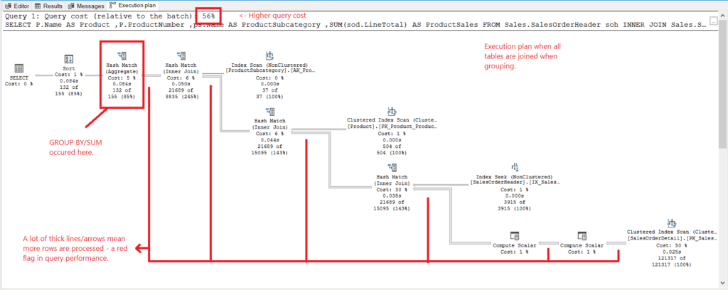
Figure 4. Execution plan when all tables are joined.
And we have the following observations:
- GROUP BY and SUM were done late in the process after joining all tables.
- A lot of thicker lines and arrows – this explains the 1,277 logical reads.
- The 2 queries combined form 100% of the query cost. But this query’s plan has a higher query cost (56%).
Now, here’s an execution plan when we group first, and joined the Product and ProductSubcategory tables later. Check out Figure 5.
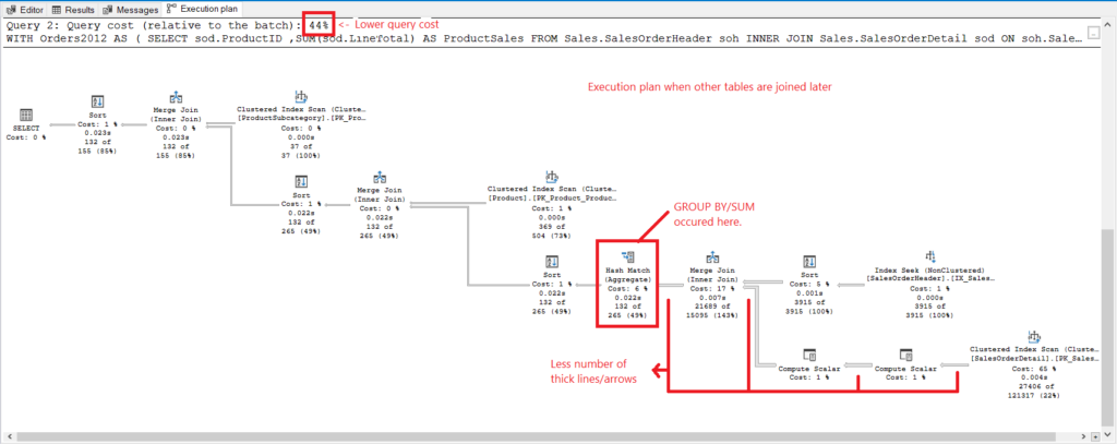
Figure 5. Execution plan when the group first, join later is done.
And we have the following observations in Figure 5.
- GROUP BY and SUM finished early.
- Less number of thick lines and arrows – this explains the 348 logical reads only.
- Lower query cost (44%).
Example 3: How Indexing Affects SQL GROUP BY Performance
Whenever SQL GROUP BY is done on a column, that column should have an index. You will increase execution speed once you group the column with an index. Let’s modify the previous query and use the ship date instead of the order date. The ship date column has no index in SalesOrderHeader.
SET STATISTICS IO ON
GO

SELECT
 MONTH(soh.ShipDate) AS ShipMonth
,YEAR(soh.ShipDate) AS ShipYear
,p.Name AS Product
,SUM(sod.LineTotal) AS ProductSales
FROM Sales.SalesOrderHeader soh
INNER JOIN Sales.SalesOrderDetail sod ON soh.SalesOrderID = sod.SalesOrderID
INNER join Production.Product p ON sod.ProductID = p.ProductID
WHERE soh.ShipDate BETWEEN '01/01/2012' AND '12/31/2012'
GROUP BY p.Name, YEAR(soh.ShipDate), MONTH(soh.ShipDate)
ORDER BY Product, ShipYear, ShipMonth;

SET STATISTICS IO OFF
GO
Press Ctrl-M, then run the query above in SSMS. Then, create a non-clustered index on the ShipDate column. Note the logical reads and execution plan. Finally, re-run the query above in another query tab. Note the differences in logical reads and execution plans.
Here’s the comparison of the logical reads in Figure 6.
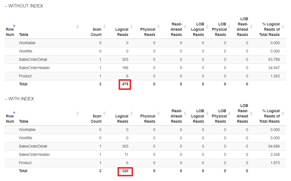
Figure 6. Logical reads of our query example with and without an index on ShipDate.
In Figure 6, there are higher logical reads of the query without an index on ShipDate.
Now let’s have the execution plan when no index on ShipDate exists in Figure 7.
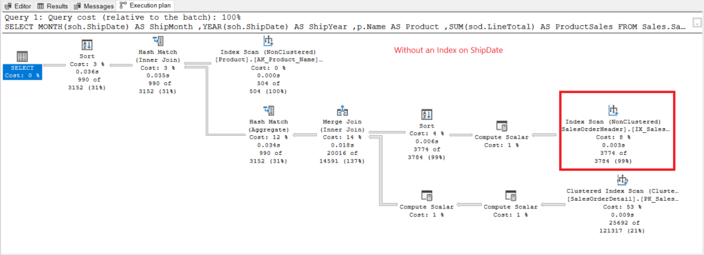
Figure 7. Execution plan when using GROUP BY on ShipDate unindexed.
The Index Scan operator used in the plan in Figure 7 explains the higher logical reads (475). Here’s an execution plan after indexing the ShipDate column.
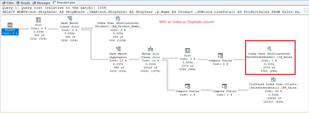
Figure 8. Execution plan when using GROUP BY on ShipDate indexed.
Instead of Index Scan, an Index Seek is used after indexing the ShipDate column. This explains the lower logical reads in Figure 6.
So, to improve the performance when using GROUP BY, consider indexing the columns you used for grouping.
Takeaways in Using SQL GROUP BY
SQL GROUP BY is easy to use. But you need to take the next step to go beyond summarizing the data for reports. Here are the points again:
- Filter early. Remove the rows you don’t need to summarize using the WHERE clause instead of the HAVING clause.
- Group first, join later. Sometimes, there will be columns you need to add aside from the columns you’re grouping. Instead of including them in the GROUP BY clause, divide the query with a CTE, and join other tables later.
- Use GROUP BY with indexed columns. This basic thing might come in handy when the database is as fast as a snail.
Hope this helps you level up your game in grouping results.
If you like this post, please share it on your favorite social media platforms.
Tags: sql functions, tips and tricks Last modified: July 17, 2023